
The
tidymodels framework is a collection of R packages for modeling and machine learning using tidyverse principles. Earlier this year, we
started regular updates here on the tidyverse blog summarizing recent developments in the tidymodels ecosystem. You can check out the
tidymodels tag to find all tidymodels blog posts here, including those that focus on a single package or more major releases. The purpose of these roundup posts is to keep you informed about any releases you may have missed and useful new functionality as we maintain these packages.
Since our last roundup post, there have been 19 CRAN releases of 15 different packages. That might sound like a lot of change to absorb as a tidymodels user! However, we purposefully write code in small, modular packages that we can release frequently to make models easier to deploy and our software easier to maintain. You can install these updates from CRAN with:
install.packages(c("broom", "butcher", "discrim", "hardhat", "parsnip", "probably",
                   "recipes", "rsample", "stacks", "themis", "tidymodels",
                   "tidyposterior", "tune", "workflowsets", "yardstick"))
The NEWS files are linked here for each package; you’ll notice that many of these releases involve small bug fixes or internal changes that are not user-facing. It’s a lot to keep up with and there are some super useful updates in the mix, so read on for several highlights!
- broom
- butcher
- discrim
- hardhat
- parsnip
- probably
- recipes
- rsample
- stacks
- themis
- tidymodels
- tidyposterior
- tune
- workflowsets
- yardstick
Reduce the memory footprint of your recipes
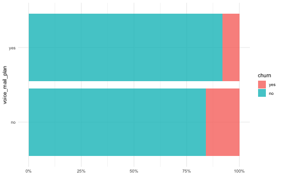
The butcher package provides methods to remove (or “axe”) components from model objects that are not needed for prediction. The most recent release updated how butcher handles recipes (the tidymodels approach for preprocessing and feature engineering) for more complete and robust coverage. Let’s consider a simulated churn-classification dataset for phone company customers:
library(tidymodels)
library(butcher)
data("mlc_churn")

set.seed(123)
churn_split <- initial_split(mlc_churn)
churn_train <- training(churn_split)
churn_test  <- testing(churn_split)

ggplot(churn_train, aes(y = voice_mail_plan, fill = churn)) +
  geom_bar(alpha = 0.8, position = "fill") +
  scale_x_continuous(labels = scales::percent_format()) +
  labs(x = NULL)
For some kinds of models, we would want to create dummy or indicator variables from nominal predictors, and preprocess features to be on the same scale. We can use recipes for this task:
churn_rec <-
  recipe(churn ~ voice_mail_plan + total_intl_minutes +
           total_day_minutes + total_eve_minutes + state,
         data = churn_train) %>%
  step_dummy(all_nominal_predictors()) %>%
  step_normalize(all_predictors())
You can prep(churn_rec) to estimate the quantities needed to create categorical features and to scale all the predictors:
churn_prep <- prep(churn_rec)
churn_prep
#> Data Recipe
#>
#> Inputs:
#>
#>       role #variables
#>    outcome          1
#>  predictor          5
#>
#> Training data contained 3750 data points and no missing data.
#>
#> Operations:
#>
#> Dummy variables from voice_mail_plan, state [trained]
#> Centering and scaling for total_intl_minutes, total_day_minutes, ... [trained]
To remove everything from this prepped recipe not needed for applying to new data (e.g.
bake() it), we can call butcher(churn_prep). In some applications, modeling practitioners need to make custom functions with a feature-engineering recipe. Sometimes those functions have… a lot of extra STUFF in them, stuff that is not needed for prediction.
butchered_plus <- function() {
  some_stuff_in_the_environment <- runif(1e6)

  churn_prep <-
    recipe(churn ~ voice_mail_plan + total_intl_minutes +
             total_day_minutes + total_eve_minutes + state,
           data = churn_train) %>%
    step_dummy(all_nominal_predictors()) %>%
    step_normalize(all_predictors()) %>%
    prep()

  butcher(churn_prep)
}
In the old version of butcher, we did not successfully remove all that extra stuff, and recipes were bigger than they needed to be:
# old version of butcher
lobstr::obj_size(butcher(churn_prep))
#> 1,835,512 B
lobstr::obj_size(butchered_plus())
#> 9,836,480 B
In the new version of butcher, we now successfully remove unneeded components from the recipe, so it is smaller:
# new version of butcher
lobstr::obj_size(butcher(churn_prep))
#> 1,695,352 B
lobstr::obj_size(butchered_plus())
#> 1,695,352 B
There are also butcher() methods for workflow() objects, so when you butcher() a modeling workflow, you remove everything not needed for prediction from both its estimated recipe and its trained model, making it as lightweight as possible for deployment.
SVMs and fast logistic regression with LiblineaR
Unfortunately, the "liquidSVM" engine for support vector machine models that parsnip supported was deprecated in the latest release, because that package was removed from CRAN. We added a new engine in the same release that allows users to fit linear SVMs with the
parsnip model svm_linear(), as well as having another option for logistic regression. This new "LiblineaR" engine is based on the same C++ library that is shipped with
scikit-learn. We’d like to thank the
maintainers of the LiblineaR R package for all their help as we set up this integration.
set.seed(234)
churn_folds <- vfold_cv(churn_train, v = 5, strata = churn)

liblinear_spec <-
  logistic_reg(penalty = 0.2, mixture = 1) %>%
  set_mode("classification") %>%
  set_engine("LiblineaR")

liblinear_wf <-
  workflow() %>%
  add_recipe(churn_rec) %>%
  add_model(liblinear_spec)

fit_resamples(liblinear_wf, resamples = churn_folds)
#> # Resampling results
#> # 5-fold cross-validation using stratification
#> # A tibble: 5 x 4
#>   splits             id    .metrics         .notes
#>   <list>             <chr> <list>           <list>
#> 1 <split [2999/751]> Fold1 <tibble [2 × 4]> <tibble [0 × 1]>
#> 2 <split [2999/751]> Fold2 <tibble [2 × 4]> <tibble [0 × 1]>
#> 3 <split [3000/750]> Fold3 <tibble [2 × 4]> <tibble [0 × 1]>
#> 4 <split [3001/749]> Fold4 <tibble [2 × 4]> <tibble [0 × 1]>
#> 5 <split [3001/749]> Fold5 <tibble [2 × 4]> <tibble [0 × 1]>
The "LiblineaR" engine for regularized logistic regression
can be very fast compared to the "glmnet" engine, even when we use a
sparse representation. Check out
benchmarking code here.
Post-processing your model predictions with probably and yardstick
We recently had releases of both the
yardstick and
probably packages, which now work together even better. The probably package can, among other things, help you post-process your model predictions. This data on churn is imbalanced, with many more customers who did not churn than those who did; we may need to use a threshold other than 0.5 for most appropriate results, or an organization may want to set a specific threshold for some action to prevent churn. You can set a threshold using the
probably function make_two_class_pred().
library(probably)

set.seed(123)
churn_preds <-
  liblinear_wf %>%
  fit(churn_train) %>%
  augment(churn_test)

churn_post <-
  churn_preds %>%
  mutate(.pred = make_two_class_pred(.pred_yes, levels(churn), threshold = 0.7))
The class predictions created with probably integrate well with functions from yardstick, including custom sets of metrics created with
metric_set().
churn_metrics <- metric_set(accuracy, sens, spec)

churn_post %>% churn_metrics(truth = churn, estimate = .pred_class)
#> # A tibble: 3 x 3
#>   .metric  .estimator .estimate
#>   <chr>    <chr>          <dbl>
#> 1 accuracy binary        0.854
#> 2 sens     binary        0.0619
#> 3 spec     binary        0.999
churn_post %>% churn_metrics(truth = churn, estimate = .pred)
#> # A tibble: 3 x 3
#>   .metric  .estimator .estimate
#>   <chr>    <chr>          <dbl>
#> 1 accuracy binary         0.746
#> 2 sens     binary         0.149
#> 3 spec     binary         0.856
Notice that with the default threshold of 0.5, basically no customers were classified as at risk for churn! Adjusting the threshold with make_two_class_pred() helps to address this issue.
Acknowledgements
We’d like to extend our thanks to all of the contributors who helped make these releases during Q2 possible!
broom: @alexpghayes, @andrewsris, @arcruz0, @bbolker, @bgall, @cccneto, @ddsjoberg, @DerForscher107, @dikiprawisuda, @dmenne, @grantmcdermott, @japhir, @karldw, @kelseygonzalez, @leejasme, @LukasWallrich, @MatthieuStigler, @mbac, @nt-williams, @pachadotdev, @rpruim, @rsbivand, @simonpcouch, and @vincentarelbundock.
butcher: @bshor, @DavisVaughan, @juliasilge, and @lbenz-mdsol.
discrim: @juliasilge, and @topepo.
hardhat: @DavisVaughan, and @topepo.
parsnip: @brshallo, @cgoo4, @DavisVaughan, @dgrtwo, @EmilHvitfeldt, @graysonwhite, @hfrick, @hsbadr, @joeycouse, @jtlandis, @juliasilge, @klin333, @mdancho84, @paulponcet, @pfc5098, @RaymondBalise, @smingerson, @topepo, @UnclAlDeveloper, and @vadimus202.
probably: @hsbadr, and @juliasilge.
recipes: @AlbertRapp, @asmae-toumi, @atusy, @christiantillich, @EdwinTh, @EmilHvitfeldt, @hfrick, @jake-mason, @jkennel, @jtlandis, @juliasilge, @LiamBlake, @lindeloev, @mikemc, @mrkaye97, @renanxcortes, @schoonees, @SlowMo24, @smingerson, and @topepo.
rsample: @brian-j-smith, @EmilHvitfeldt, @hfrick, @juliasilge, @LiamBlake, @mattwarkentin, @PathosEthosLogos, @rkb965, and @supermdat.
stacks: @asmae-toumi, @Crisel12, @simonpcouch, and @topepo.
themis: @EmilHvitfeldt, @kylegilde, and @topepo.
tidymodels: @dmenne, @Edward-Egros, @juliasilge, @PathosEthosLogos, @topepo, and @verajosemanuel.
tidyposterior: @juliasilge, and @topepo.
tune: @albert-ying, @amazongodman, @brshallo, @dpanyard, @EmilHvitfeldt, @juliasilge, @klin333, @mbac, @PathosEthosLogos, @silvanhi, @smingerson, @topepo, and @yogat3ch.
workflowsets: @amazongodman, @DavisVaughan, @gunnergalactico, @hnagaty, @jonthegeek, @juliasilge, @mdancho84, @oskasf, @rafzamb, @topepo, and @yogat3ch.
yardstick: @brshallo, @coletl, @datenzauberai, @DavisVaughan, @EmilHvitfeldt, @juliasilge, @klin333, @mattwarkentin, @mdancho84, and @topepo.