
Another year, another roundup of tidyverse updates, through the lens of an educator. As with previous teaching the tidyverse posts, much of what is discussed in this blog post has already been covered in package update posts, however the goal of this roundup is to summarize the highlights that are most relevant to teaching data science with the tidyverse, particularly to new learners.
Specifically, I’ll discuss:
- Resource refresh
- Nine core packages in tidyverse 2.0.0
- Conflict resolution in the tidyverse
- Improved and expanded
*_join()functionality - Per operation grouping
- Quality of life improvements to
case_when()andif_else() - New syntax for separating columns
- New argument for line geoms: linewidth
- Other highlights
- Coming up
And different from previous posts on this topic, this one comes with a video! If you’d like a live demo of the code examples, and a few more additional tips along the way, you can watch the video below.
Throughout this blog post you’ll encounter some code chunks with the comment previously, indicating what you used to do in the tidyverse. Often these will be coupled with chunks with the comment now, optionally, indicating what you can now do with the tidyverse. And rarely, they will be coupled with chunks with the comment now, indicating what you should do instead now with the tidyverse.
Let’s get started with the obligatory…
library(tidyverse)
#> ── Attaching core tidyverse packages ──────────────────────── tidyverse 2.0.0 ──
#> ✔ dplyr     1.1.2     ✔ readr     2.1.4
#> ✔ forcats   1.0.0     ✔ stringr   1.5.0
#> ✔ ggplot2   3.4.2     ✔ tibble    3.2.1
#> ✔ lubridate 1.9.2     ✔ tidyr     1.3.0
#> ✔ purrr     1.0.1
#> ── Conflicts ────────────────────────────────────────── tidyverse_conflicts() ──
#> ✖ dplyr::filter() masks stats::filter()
#> ✖ dplyr::lag()    masks stats::lag()
#> ℹ Use the conflicted package (<http://conflicted.r-lib.org/>) to force all conflicts to become errors
And, let’s also load the palmerpenguins package that we will use in examples.
Resource refresh
R for Data Science, 2nd Edition is out! This blog post (and the book’s preface) outlines updates since the first edition. Updates to the book served as the motivation for many of the changes mentioned in the remainder of this post as as well as on the Tidyverse blog over the last year. Now that the book is out, you can expect the pace of change to slow down again for a while, which means plenty of time for phasing these changes into your teaching materials.
One change in the 2nd Edition that will most likely affect almost all of your teaching materials is the use of the native R pipe (|>) instead of the magrittr pipe (%>%). If you’re not familiar with the similarities and differences between these operators, I recommend reading
this comparison blog post. And I strongly recommend making this update since it will allow students to perform piped operations with any R function, and hence allow them to keep their data pipeline workflows regardless of whether the next package they learn is from the tidyverse (or package that uses tidyverse principles) or not.
Nine core packages in tidyverse 2.0.0
The main update in tidyverse 2.0.0, which was released in March 2023, is that it lubridate is now a core tidyverse package. The lubridate package that makes it easier to do the things R does with date-times, is now a core tidyverse package. So, while many of your scripts in the past may have started with
you can now just do
and the lubridate package will be loaded as well.
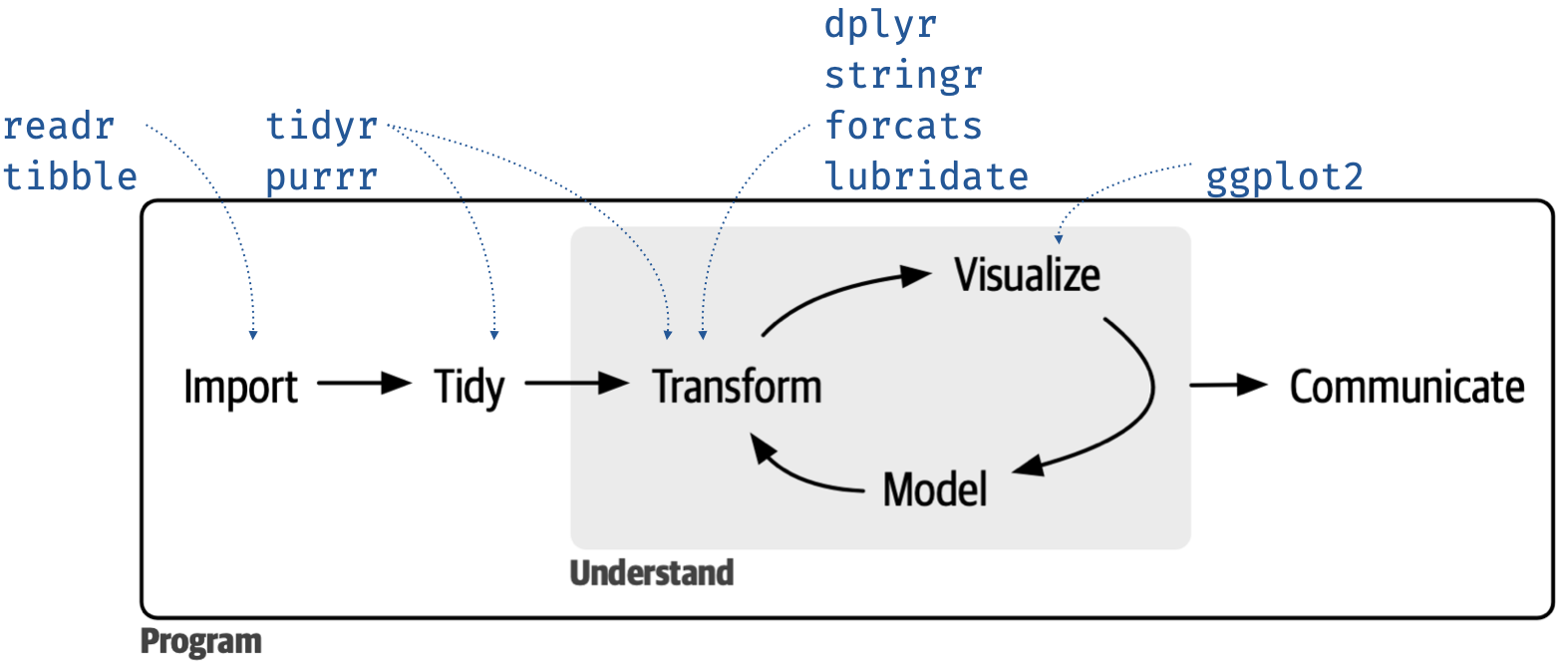
If you, like me, use a graphic like the one below that maps the core tidyverse packages to phases of the data science cycle, here is an updated graphic including lubridate.
Conflict resolution in the tidyverse
You may have also noticed that the package loading message for the tidyverse has been updated as well, and now advertises the conflicted package.
#> ── Conflicts ────────────────────────────────────────── tidyverse_conflicts() ──
#> ✖ dplyr::filter() masks stats::filter()
#> ✖ dplyr::lag()    masks stats::lag()
#> ℹ Use the conflicted package (<http://conflicted.r-lib.org/>) to force all conflicts to become errors
Conflict resolution in R, i.e., what to do if multiple packages that are loaded in a session have functions with the same name, can get tricky, and the conflicted package is designed to help with that. R’s default conflict resolution gives precedence to the most recently loaded package. For example, if you use the filter function before loading the tidyverse, R will use
stats::filter():
penguins |>
  filter(species == "Adelie")
#> Error in eval(expr, envir, enclos): object 'species' not found
However, after loading the tidyverse, when you call
filter(), R will silently choose
dplyr::filter():
penguins |>
  filter(species == "Adelie")
#> # A tibble: 152 × 8
#>    species island    bill_length_mm bill_depth_mm flipper_length_mm body_mass_g
#>    <fct>   <fct>              <dbl>         <dbl>             <int>       <int>
#>  1 Adelie  Torgersen           39.1          18.7               181        3750
#>  2 Adelie  Torgersen           39.5          17.4               186        3800
#>  3 Adelie  Torgersen           40.3          18                 195        3250
#>  4 Adelie  Torgersen           NA            NA                  NA          NA
#>  5 Adelie  Torgersen           36.7          19.3               193        3450
#>  6 Adelie  Torgersen           39.3          20.6               190        3650
#>  7 Adelie  Torgersen           38.9          17.8               181        3625
#>  8 Adelie  Torgersen           39.2          19.6               195        4675
#>  9 Adelie  Torgersen           34.1          18.1               193        3475
#> 10 Adelie  Torgersen           42            20.2               190        4250
#> # ℹ 142 more rows
#> # ℹ 2 more variables: sex <fct>, year <int>
This silent conflict resolution approach works fine until it doesn’t, and then it can be very frustrating to debug. The conflicted package does not allow for silent conflict resolution:
library(conflicted)

penguins |>
  filter(species == "Adelie")
#> Error:
#> ! [conflicted] filter found in 2 packages.
#> Either pick the one you want with `::`:
#> • dplyr::filter
#> • stats::filter
#> Or declare a preference with `conflicts_prefer()`:
#> • `conflicts_prefer(dplyr::filter)`
#> • `conflicts_prefer(stats::filter)`
You can, of course, use
dplyr::filter() but if you have a bunch of data wrangling pipelines, which is likely the case if you’re teaching data wrangling, it can get pretty busy.
Instead, with conflicted, you can explicitly declare which
filter() you want to use at the beginning (of a session, of a script, or of an R Markdown or Quarto file) with
conflicts_prefer():
conflicts_prefer(dplyr::filter)
#> [conflicted] Will prefer dplyr::filter over any other package.

penguins |>
  filter(species == "Adelie")
#> # A tibble: 152 × 8
#>    species island    bill_length_mm bill_depth_mm flipper_length_mm body_mass_g
#>    <fct>   <fct>              <dbl>         <dbl>             <int>       <int>
#>  1 Adelie  Torgersen           39.1          18.7               181        3750
#>  2 Adelie  Torgersen           39.5          17.4               186        3800
#>  3 Adelie  Torgersen           40.3          18                 195        3250
#>  4 Adelie  Torgersen           NA            NA                  NA          NA
#>  5 Adelie  Torgersen           36.7          19.3               193        3450
#>  6 Adelie  Torgersen           39.3          20.6               190        3650
#>  7 Adelie  Torgersen           38.9          17.8               181        3625
#>  8 Adelie  Torgersen           39.2          19.6               195        4675
#>  9 Adelie  Torgersen           34.1          18.1               193        3475
#> 10 Adelie  Torgersen           42            20.2               190        4250
#> # ℹ 142 more rows
#> # ℹ 2 more variables: sex <fct>, year <int>
Getting back to the package loading message… It can be tempting, particularly in a teaching scenario, particularly to an audience of new learners, and particularly if you teach with slides and messages take up valuable slide real estate, I would urge you to not hide startup messages from teaching materials. Instead, address them early on to:
Encourage reading and understanding messages, warnings, and errors – teaching people to read error messages is hard enough, it’s going to be even harder if you’re not modeling that to them.
Help during hard-to-debug situations resulting from base R’s silent conflict resolution – because, let’s face it, someone in your class, if not you during a live-coding session, will see that pesky object not found error at some point when using
filter().
Improved and expanded *_join() functionality
The
dplyr package has long had the
*_join() family of functions for joining data frames. dplyr 1.1.0 introduced a
bunch of extensions that bring joins closer to the power available in other systems like SQL and data.table.
join_by()
New functionality for join functions includes a new
join_by() function for the by argument. So, while in the past your code may have looked like the following:
# previously
*_join(
  x, y,
  by = c("" = "")
)
you can now do:
# now, optionally
*_join(
  x, y,
  by = join_by( == )
)
For example, suppose you have the following information on the three islands we have penguins from:
islands <- tribble(
  ~name,       ~coordinates,
  "Torgersen", "64°46′S 64°5′W",
  "Biscoe",    "65°26′S 65°30′W",
  "Dream",     "64°44′S 64°14′W"
)

islands
#> # A tibble: 3 × 2
#>   name      coordinates
#>   <chr>     <chr>
#> 1 Torgersen 64°46′S 64°5′W
#> 2 Biscoe    65°26′S 65°30′W
#> 3 Dream     64°44′S 64°14′W
You can join this to the penguins data frame by matching the island column in the penguins data frame to the name column in the islands data frame:
penguins |>
  left_join(
    islands,
    by = join_by(island == name)
  ) |>
  select(species, island, coordinates)
#> # A tibble: 344 × 3
#>    species island    coordinates
#>    <fct>   <chr>     <chr>
#>  1 Adelie  Torgersen 64°46′S 64°5′W
#>  2 Adelie  Torgersen 64°46′S 64°5′W
#>  3 Adelie  Torgersen 64°46′S 64°5′W
#>  4 Adelie  Torgersen 64°46′S 64°5′W
#>  5 Adelie  Torgersen 64°46′S 64°5′W
#>  6 Adelie  Torgersen 64°46′S 64°5′W
#>  7 Adelie  Torgersen 64°46′S 64°5′W
#>  8 Adelie  Torgersen 64°46′S 64°5′W
#>  9 Adelie  Torgersen 64°46′S 64°5′W
#> 10 Adelie  Torgersen 64°46′S 64°5′W
#> # ℹ 334 more rows
While by = c("island" = "name") would still work, I would recommend teaching
join_by() over by so that:
- You can read it out loud as “where x is equal to y”, just like in other logical statements where
==is pronounced as “is equal to”. - You don’t have to worry about
by = c(x = y)(which is invalid) vs.by = c(x = "y")(which is valid) vs.by = c("x" = "y")(which is also valid).
In fact, for succinctness, you might avoid the argument name and express this as:
Handling various matches
The *_join() functions now have additional arguments for handling multiple matches and unmatched rows as well as for specifying the relationship between the two data frames.
So, while in the past your code may have looked like the following:
# previously
*_join(
  x, y, by
)
you can now do:
# now, optionally
*_join(
  x, y, by,
  multiple = "all",
  unmatched = "drop",
  relationship = NULL
)
Let’s set up three data frames to demonstrate the new functionality:
- Information about three penguins, one row per
samp_id:
three_penguins <- tribble(
  ~samp_id, ~species,    ~island,
  1,        "Adelie",    "Torgersen",
  2,        "Gentoo",    "Biscoe",
  3,        "Chinstrap", "Dream"
)

three_penguins
#> # A tibble: 3 × 3
#>   samp_id species   island
#>     <dbl> <chr>     <chr>
#> 1       1 Adelie    Torgersen
#> 2       2 Gentoo    Biscoe
#> 3       3 Chinstrap Dream
- Information about weight measurements of these penguins, one row per
samp_id,meas_idcombination:
weight_measurements <- tribble(
  ~samp_id, ~meas_id, ~body_mass_g,
  1,        1,        3220,
  1,        2,        3250,
  2,        1,        4730,
  2,        2,        4725,
  3,        1,        4000,
  3,        2,        4050
)

weight_measurements
#> # A tibble: 6 × 3
#>   samp_id meas_id body_mass_g
#>     <dbl>   <dbl>       <dbl>
#> 1       1       1        3220
#> 2       1       2        3250
#> 3       2       1        4730
#> 4       2       2        4725
#> 5       3       1        4000
#> 6       3       2        4050
- Information about flipper measurements of these penguins, one row per
samp_id,meas_idcombination:
flipper_measurements <- tribble(
  ~samp_id, ~meas_id, ~flipper_length_mm,
  1,        1,        193,
  1,        2,        195,
  2,        1,        214,
  2,        2,        216,
  3,        1,        203,
  3,        2,        203
)

flipper_measurements
#> # A tibble: 6 × 3
#>   samp_id meas_id flipper_length_mm
#>     <dbl>   <dbl>             <dbl>
#> 1       1       1               193
#> 2       1       2               195
#> 3       2       1               214
#> 4       2       2               216
#> 5       3       1               203
#> 6       3       2               203
One-to-many relationships don’t require extra care, they just work:
three_penguins |>
  left_join(weight_measurements, join_by(samp_id))
#> # A tibble: 6 × 5
#>   samp_id species   island    meas_id body_mass_g
#>     <dbl> <chr>     <chr>       <dbl>       <dbl>
#> 1       1 Adelie    Torgersen       1        3220
#> 2       1 Adelie    Torgersen       2        3250
#> 3       2 Gentoo    Biscoe          1        4730
#> 4       2 Gentoo    Biscoe          2        4725
#> 5       3 Chinstrap Dream           1        4000
#> 6       3 Chinstrap Dream           2        4050
However, many-to-many relationships require some extra care. For example, if we join the three_penguins data frame to the flipper_measurements data frame, we get a warning:
weight_measurements |>
  left_join(flipper_measurements, join_by(samp_id))
#> Warning in left_join(weight_measurements, flipper_measurements, join_by(samp_id)): Detected an unexpected many-to-many relationship between `x` and `y`.
#> ℹ Row 1 of `x` matches multiple rows in `y`.
#> ℹ Row 1 of `y` matches multiple rows in `x`.
#> ℹ If a many-to-many relationship is expected, set `relationship =
#>   "many-to-many"` to silence this warning.
#> # A tibble: 12 × 5
#>    samp_id meas_id.x body_mass_g meas_id.y flipper_length_mm
#>      <dbl>     <dbl>       <dbl>     <dbl>             <dbl>
#>  1       1         1        3220         1               193
#>  2       1         1        3220         2               195
#>  3       1         2        3250         1               193
#>  4       1         2        3250         2               195
#>  5       2         1        4730         1               214
#>  6       2         1        4730         2               216
#>  7       2         2        4725         1               214
#>  8       2         2        4725         2               216
#>  9       3         1        4000         1               203
#> 10       3         1        4000         2               203
#> 11       3         2        4050         1               203
#> 12       3         2        4050         2               203
We get a warning about unexpected many-to-many relationships (unexpected because we didn’t specify this type of relationship in our join call), and the warning suggests setting relationship = "many-to-many". And note that we went from 6 rows (measurements) to 12, which is also unexpected.
weight_measurements |>
  left_join(flipper_measurements, join_by(samp_id), relationship = "many-to-many")
#> # A tibble: 12 × 5
#>    samp_id meas_id.x body_mass_g meas_id.y flipper_length_mm
#>      <dbl>     <dbl>       <dbl>     <dbl>             <dbl>
#>  1       1         1        3220         1               193
#>  2       1         1        3220         2               195
#>  3       1         2        3250         1               193
#>  4       1         2        3250         2               195
#>  5       2         1        4730         1               214
#>  6       2         1        4730         2               216
#>  7       2         2        4725         1               214
#>  8       2         2        4725         2               216
#>  9       3         1        4000         1               203
#> 10       3         1        4000         2               203
#> 11       3         2        4050         1               203
#> 12       3         2        4050         2               203
With relationship = "many-to-many", we no longer get a warning. However, the “explosion of rows” issue is still there. Addressing that requires rethinking what we join the two data frames by:
weight_measurements |>
  left_join(flipper_measurements, join_by(samp_id, meas_id))
#> # A tibble: 6 × 4
#>   samp_id meas_id body_mass_g flipper_length_mm
#>     <dbl>   <dbl>       <dbl>             <dbl>
#> 1       1       1        3220               193
#> 2       1       2        3250               195
#> 3       2       1        4730               214
#> 4       2       2        4725               216
#> 5       3       1        4000               203
#> 6       3       2        4050               203
We can see that while the warning nudged us towards setting relationship = "many-to-many", turns out the correct way to address the problem was to join by both samp_id and meas_id.
We’ll wrap up our discussion on new functionality for handling unmatched cases. We’ll create one more data frame (four_penguins) to exemplify this:
four_penguins <- tribble(
  ~samp_id, ~species,    ~island,
  1,        "Adelie",    "Torgersen",
  2,        "Gentoo",    "Biscoe",
  3,        "Chinstrap", "Dream",
  4,        "Adelie",    "Biscoe"
)

four_penguins
#> # A tibble: 4 × 3
#>   samp_id species   island
#>     <dbl> <chr>     <chr>
#> 1       1 Adelie    Torgersen
#> 2       2 Gentoo    Biscoe
#> 3       3 Chinstrap Dream
#> 4       4 Adelie    Biscoe
If we just join weight_measurements to four_penguins, the unmatched fourth penguin silently disappears, which is less than ideal, particularly in a more realistic scenario with many more observations:
weight_measurements |>
  left_join(four_penguins, join_by(samp_id))
#> # A tibble: 6 × 5
#>   samp_id meas_id body_mass_g species   island
#>     <dbl>   <dbl>       <dbl> <chr>     <chr>
#> 1       1       1        3220 Adelie    Torgersen
#> 2       1       2        3250 Adelie    Torgersen
#> 3       2       1        4730 Gentoo    Biscoe
#> 4       2       2        4725 Gentoo    Biscoe
#> 5       3       1        4000 Chinstrap Dream
#> 6       3       2        4050 Chinstrap Dream
Setting unmatched = "error" protects you from accidentally dropping rows:
weight_measurements |>
  left_join(four_penguins, join_by(samp_id), unmatched = "error")
#> Error in `left_join()`:
#> ! Each row of `y` must be matched by `x`.
#> ℹ Row 4 of `y` was not matched.
Once you see the error message, you can decide how to handle the unmatched rows, e.g., explicitly drop them.
weight_measurements |>
  left_join(four_penguins, join_by(samp_id), unmatched = "drop")
#> # A tibble: 6 × 5
#>   samp_id meas_id body_mass_g species   island
#>     <dbl>   <dbl>       <dbl> <chr>     <chr>
#> 1       1       1        3220 Adelie    Torgersen
#> 2       1       2        3250 Adelie    Torgersen
#> 3       2       1        4730 Gentoo    Biscoe
#> 4       2       2        4725 Gentoo    Biscoe
#> 5       3       1        4000 Chinstrap Dream
#> 6       3       2        4050 Chinstrap Dream
There are many more developments related to *_join() functions (e.g.,
inequality joins and
rolling joins), but many of these likely wouldn’t come up in an introductory course so we won’t get into their details. A good place to read more about them is
R for Data Science, 2nd edition.
Exploding joins (i.e., joins that result in a larger number of rows than either of the data frames from bie) can be hard to debug for students! Teaching them the tools to diagnose whether the join they performed, and that may not have given an error, is indeed the one they wanted to perform. Did they lose any cases? Did they gain an unexpected amount of cases? Did they perform a join without thinking and take down the entire teaching server? These things happen, particularly if students are working with their own data for an open-ended project!
Per operation grouping
To calculate grouped summary statistics, you previously needed to do something like this:
Now, an alternative approach is to pass the groups directly in the
summarize() call:
Let’s take a look at the differences between these two approaches before making a recommendation for one over the other.
group_by() can result in groups that persist in the output, particularly when grouping by multiple variables. For example, in the following pipeline we group the penguins data frame by species and sex, find mean body weights for each resulting species / sex combination, and then show the first observation in the output with slice_head(n = 1). Since the output is grouped by species, this results in one summary statistic per species.
penguins |>
  drop_na(sex, body_mass_g) |>
  group_by(species, sex) |>
  summarize(mean_bw = mean(body_mass_g)) |>
  slice_head(n = 1)
#> `summarise()` has grouped output by 'species'. You can override using the
#> `.groups` argument.
#> # A tibble: 3 × 3
#> # Groups:   species [3]
#>   species   sex    mean_bw
#>   <fct>     <fct>    <dbl>
#> 1 Adelie    female   3369.
#> 2 Chinstrap female   3527.
#> 3 Gentoo    female   4680.
If we explicitly drop the groups in the
summarize() call, so that the output is no longer grouped, we get just one row in our output.
penguins |>
  drop_na(sex, body_mass_g) |>
  group_by(species, sex) |>
  summarize(mean_bw = mean(body_mass_g), .groups = "drop") |>
  slice_head(n = 1)
#> # A tibble: 1 × 3
#>   species sex    mean_bw
#>   <fct>   <fct>    <dbl>
#> 1 Adelie  female   3369.
This pair of examples show that whether your output is grouped or not can affect downstream results, and if you’re a
group_by() user, you’ve probably been burnt by this once or twice.
Per-operation grouping allows you to define groups in a .by argument, and these groups don’t persist. So, regardless of whether you group by one or two variables, the resulting data frame after calculating a summary statistic is not grouped.
# group by 1 variable
penguins |>
  drop_na(sex, body_mass_g) |>
  summarize(
    mean_bw = mean(body_mass_g),
    .by = species
  )
#> # A tibble: 3 × 2
#>   species   mean_bw
#>   <fct>       <dbl>
#> 1 Adelie      3706.
#> 2 Gentoo      5092.
#> 3 Chinstrap   3733.

# group by 2 variables
penguins |>
  drop_na(sex, body_mass_g) |>
  summarize(
    mean_bw = mean(body_mass_g),
    .by = c(species, sex)
  )
#> # A tibble: 6 × 3
#>   species   sex    mean_bw
#>   <fct>     <fct>    <dbl>
#> 1 Adelie    male     4043.
#> 2 Adelie    female   3369.
#> 3 Gentoo    female   4680.
#> 4 Gentoo    male     5485.
#> 5 Chinstrap female   3527.
#> 6 Chinstrap male     3939.
So, when teaching grouped operations, you now have the option to choose between these two approaches. The most important teaching tip I can give, particularly for teaching to new learners, is to choose one method and stick to it. The .by method will result in fewer outputs that are unintentionally grouped, and hence, might potentially be easier for new learners. And while this approach is mentioned in R for Data Science, 2nd edition, the
group_by() approach is described in more detail.
On the other hand. for more experienced learners, particularly those learning to design their own functions and packages, the evolution of grouping in the tidyverse can be an interesting subject to review.
Quality of life improvements to case_when() and if_else()
case_when()
Previously, when writing a
case_when() statement, you had to use TRUE to indicate “all else”. Additionally,
case_when() has historically been strict about the types on the right-hand side, e.g., requiring NA_character when other right-hand side values are characters, and not letting you get away with just NA.
# previously
df |>
  mutate(
    x = case_when(
       ~ "value 1",
       ~ "value 2",
       ~ "value 3",
      TRUE          ~ NA_character_
    )
  )
Now, optionally, you can define “all else” in a .default argument of
case_when() and you no longer need to worry about the type of NA you use on the right-hand side.
# now, optionally
df |>
  mutate(
    x = case_when(
       ~ "value 1",
       ~ "value 2",
       ~ "value 3",
      .default = NA
    )
  )
For example, you can now do something like the following when creating a categorical version of a numerical variable that has some NAs.
penguins |>
  mutate(
    bm_cat = case_when(
      is.na(body_mass_g) ~ NA,
      body_mass_g < 3550 ~ "Small",
      between(body_mass_g, 3550, 4750) ~ "Medium",
      .default = "Large"
    )
  ) |>
  relocate(body_mass_g, bm_cat)
#> # A tibble: 344 × 9
#>    body_mass_g bm_cat species island    bill_length_mm bill_depth_mm
#>          <int> <chr>  <fct>   <fct>              <dbl>         <dbl>
#>  1        3750 Medium Adelie  Torgersen           39.1          18.7
#>  2        3800 Medium Adelie  Torgersen           39.5          17.4
#>  3        3250 Small  Adelie  Torgersen           40.3          18
#>  4          NA NA     Adelie  Torgersen           NA            NA
#>  5        3450 Small  Adelie  Torgersen           36.7          19.3
#>  6        3650 Medium Adelie  Torgersen           39.3          20.6
#>  7        3625 Medium Adelie  Torgersen           38.9          17.8
#>  8        4675 Medium Adelie  Torgersen           39.2          19.6
#>  9        3475 Small  Adelie  Torgersen           34.1          18.1
#> 10        4250 Medium Adelie  Torgersen           42            20.2
#> # ℹ 334 more rows
#> # ℹ 3 more variables: flipper_length_mm <int>, sex <fct>, year <int>
if_else()
Similarly,
if_else() is no longer as strict about typed missing values either.
penguins |>
  mutate(
    bm_unit = if_else(!is.na(body_mass_g), paste(body_mass_g, "g"), NA)
  ) |>
  relocate(body_mass_g, bm_unit)
#> # A tibble: 344 × 9
#>    body_mass_g bm_unit species island    bill_length_mm bill_depth_mm
#>          <int> <chr>   <fct>   <fct>              <dbl>         <dbl>
#>  1        3750 3750 g  Adelie  Torgersen           39.1          18.7
#>  2        3800 3800 g  Adelie  Torgersen           39.5          17.4
#>  3        3250 3250 g  Adelie  Torgersen           40.3          18
#>  4          NA NA      Adelie  Torgersen           NA            NA
#>  5        3450 3450 g  Adelie  Torgersen           36.7          19.3
#>  6        3650 3650 g  Adelie  Torgersen           39.3          20.6
#>  7        3625 3625 g  Adelie  Torgersen           38.9          17.8
#>  8        4675 4675 g  Adelie  Torgersen           39.2          19.6
#>  9        3475 3475 g  Adelie  Torgersen           34.1          18.1
#> 10        4250 4250 g  Adelie  Torgersen           42            20.2
#> # ℹ 334 more rows
#> # ℹ 3 more variables: flipper_length_mm <int>, sex <fct>, year <int>
While these may be seemingly small improvements, I think they have huge benefits for teaching and learning. It’s a blessing to not have to introduce NA_character_ and friends as early as introducing
if_else() and
case_when()! Different types of NAs are a good topic for a course on R as a programming language, statistical computing, etc. but they are unnecessarily complex for an introductory course.
New syntax for separating columns
The following table summarizes new syntax for separating columns in tidyr that supersede
extract(),
separate(), and
separate_rows(). These updates are motivated by the goal of achieving a set of functions that have more consistent names and arguments, have better performance, and provide a new approach for handling problems:
| MAKE COLUMNS | MAKE ROWS | |
|---|---|---|
| Separate with delimiter | separate_wider_delim() | separate_longer_delim() |
| Separate by position | separate_wider_position() | separate_longer_position() |
| Separate with regular expression |
Here is an example for using some of these functions. Let’s suppose we have data on three penguins with their descriptions.
three_penguin_descriptions <- tribble(
  ~id, ~description,
  1,   "Species: Adelie, Island - Torgersen",
  2,   "Species: Gentoo, Island - Biscoe",
  3,   "Species: Chinstrap, Island - Dream",
)

three_penguin_descriptions
#> # A tibble: 3 × 2
#>      id description
#>   <dbl> <chr>
#> 1     1 Species: Adelie, Island - Torgersen
#> 2     2 Species: Gentoo, Island - Biscoe
#> 3     3 Species: Chinstrap, Island - Dream
We can seaprate the description column into species and island with
separate_wider_delim():
three_penguin_descriptions |>
  separate_wider_delim(
    cols = description,
    delim = ", ",
    names = c("species", "island")
  )
#> # A tibble: 3 × 3
#>      id species            island
#>   <dbl> <chr>              <chr>
#> 1     1 Species: Adelie    Island - Torgersen
#> 2     2 Species: Gentoo    Island - Biscoe
#> 3     3 Species: Chinstrap Island - Dream
Or we can do so with regular expressions:
three_penguin_descriptions |>
  separate_wider_regex(
    cols = description,
    patterns = c(
      "Species: ", species = "[^,]+",
      ", ",
      "Island - ", island = ".*"
    )
  )
#> # A tibble: 3 × 3
#>      id species   island
#>   <dbl> <chr>     <chr>
#> 1     1 Adelie    Torgersen
#> 2     2 Gentoo    Biscoe
#> 3     3 Chinstrap Dream
If teaching folks coming from doing data manipulation in spreadsheets, leverage that to motivate different types of separate_*() functions, and show the benefits of programming over point-and-click software for more advanced operations like separating longer and separating with regular expressions.
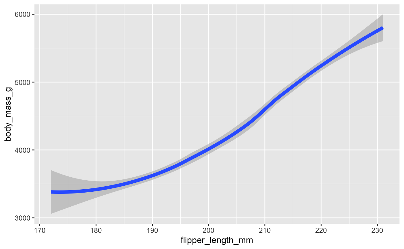
New argument for line geoms: linewidth
If you, like me, have a bunch of scatterplots with smooth lines overlaid on them, you might run into the following warning.
# previously
penguins |>
  drop_na() |>
  ggplot(aes(x = flipper_length_mm, y = body_mass_g)) +
  geom_smooth(size = 2)
#> Warning: Using `size` aesthetic for lines was deprecated in ggplot2 3.4.0.
#> ℹ Please use `linewidth` instead.
#> This warning is displayed once every 8 hours.
#> Call `lifecycle::last_lifecycle_warnings()` to see where this warning was
#> generated.
#> `geom_smooth()` using method = 'loess' and formula = 'y ~ x'

Instead of size, you should now be using linewidth.
# now
penguins |>
  drop_na() |>
  ggplot(aes(x = flipper_length_mm, y = body_mass_g)) +
  geom_smooth(linewidth = 2)
#> `geom_smooth()` using method = 'loess' and formula = 'y ~ x'
The teaching tip should be obvious here… Check the output of your old teaching materials thoroughly to not make a fool of yourself when teaching! 🤣
Other highlights
purrr 1.0.0: While purrr is likely not a common topic in introductory data science curricula, if you do teach iteration with purrr, you’ll want to check out the purrr 1.0.0 blog post. I also highly recommend Hadley’s purrr video to those who are new to purrr as well as those who want to quickly review most recent updates to it.
webR 0.1.0: webR provides a framework for creating websites where users can run R code directly within the web browser, without R installed on their device or a supporting computational R server. This is hugely exciting for writing educational materials, like interactive lesson notes, and there’s already a Quarto extension that allows you to do this: https://github.com/coatless/quarto-webr. I think this is an important space to watch for educators!
Coming up
I will be teaching a “Teaching Data Science Masterclass” at posit::conf(2023), with a module specifically on teaching the Tidyverse. Watch the course trailer and read the full course description if you’d like to find out more and sign up!