ggplot2 3.5.0: Legends

We are pleased to release ggplot2 3.5.0. This is one blogpost among several outlining changes to legend guides. Please find the main release post to read about other changes.

Legends, alongside axes, are visual representations of scales and allow observes to translate graphical properties of a plot into information. To no surprise, legends in ggplot2 comprise the guides called guide_legend(), but also guide_colourbar(), guide_coloursteps() and guide_bins().

Styling

One of the more user-visible changes is that these guides no longer have styling options. Or at least, they have been soft-deprecated: they continue to work for now, but are scheduled for removal. Gone are the days where there were 4 possible ways to set the horizontal justification of legend text in 5 different functions. There is only one way to style guides now, and that is by using theme(). The theme() function has new arguments to control the appearance of legends, which makes it easier to globally control the appearance of legends. For example: theme(legend.frame) replaces guide_colourbar(frame.colour, frame.linewidth, frame.linetype) and theme(legend.axis.line) replaces guide_bins(axis, axis.colour, axis.linewidth, axis.arrow). To allow for tweaking the style of any individual guide, the guide functions now have a theme argument that can accept a theme specific to that guide.

library(ggplot2)

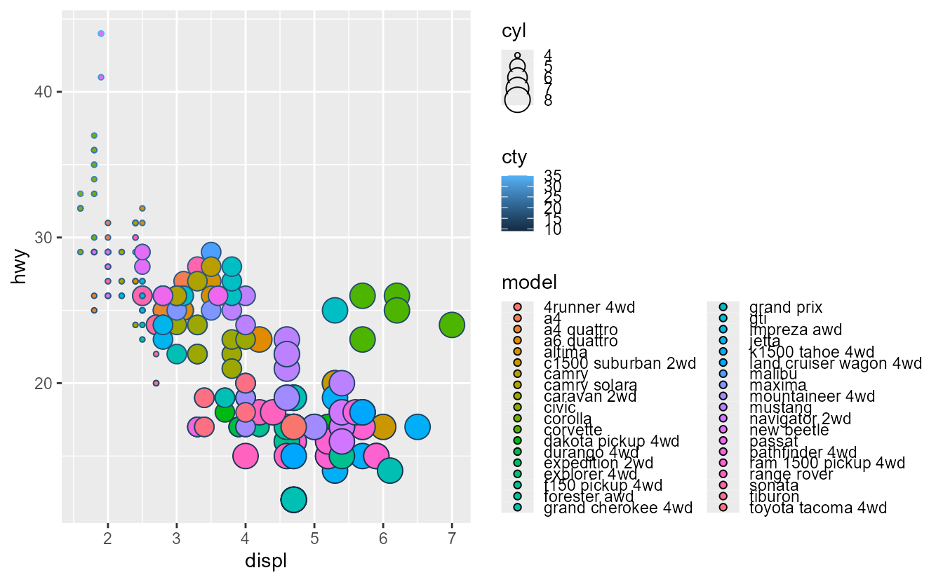
ggplot(mpg, aes(displ, hwy, shape = factor(cyl), colour = cty)) +
  geom_point() +
  # Styling individual guides
  guides(
    shape  = guide_legend(theme = theme(legend.text = element_text(colour = "red"))),
    colour = guide_colorbar(theme = theme(legend.frame = element_rect(colour = "red")))
  ) +
  # Styling guides globally
  theme(
    legend.title.position = "left",
    # Title justification is controlled by hjust/vjust in the element
    legend.title = element_text(angle = 90, hjust = 0.5)
  )

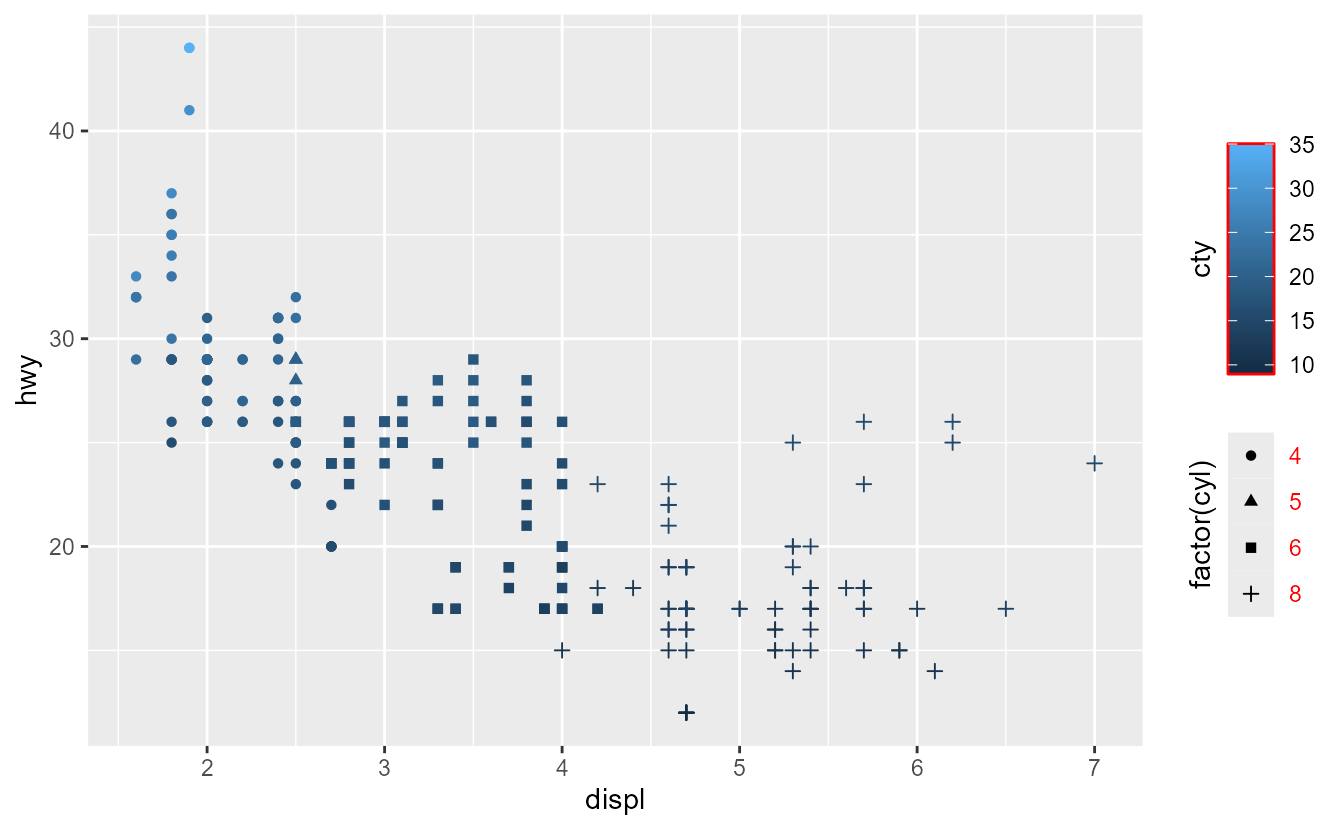
Scatterplot of engine displacement versus highway miles per gallon. The legend indicating shapes for the number of cylinders has red text. The colour bar indicating city miles per gallon has a red rectangle around the bar. Both the legend and colour bar titles are rotated, centered and on the left of the guide.

In the plot above, notice how the legend title settings affect both the colour bar and the legend, whereas the local options, like red legend text, only apply to a single guide.

Awareness

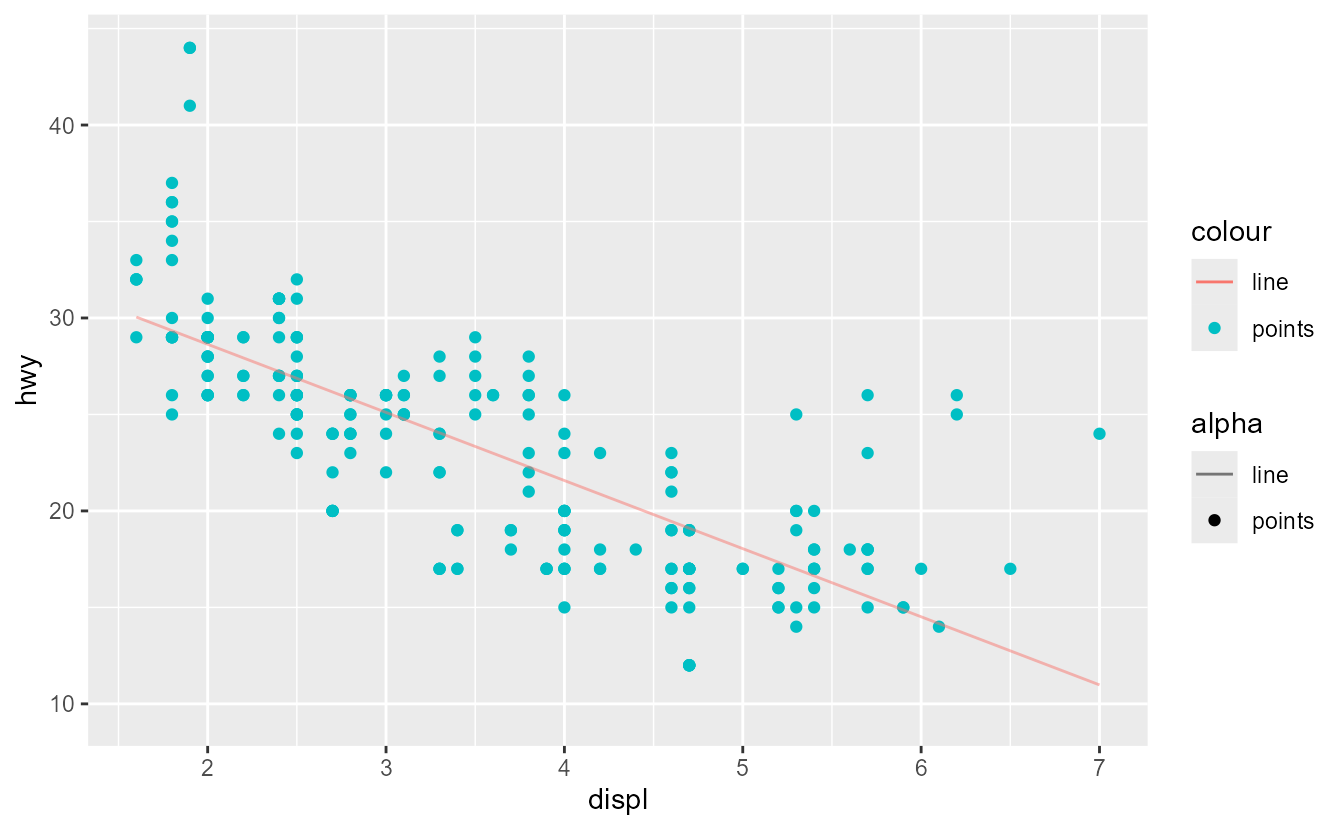
Legends are now more aware what discrete variables should be placed in which keys. By default, they now only draw keys for the layer which contain the relevant value. This saves one having to hassle with the guide_legend(override.aes) argument to get the keys to display just right. In the plot below, notice how the points and line have separate keys.

p <- ggplot(mpg, aes(displ, hwy)) +
  scale_alpha_manual(values = c(0.5, 1))
p +
  geom_point(aes(colour = "points", alpha = "points")) +
  geom_line(
    aes(colour = "line", alpha = "line"),
    stat = "smooth", formula = y ~ x, method = "lm"
  )

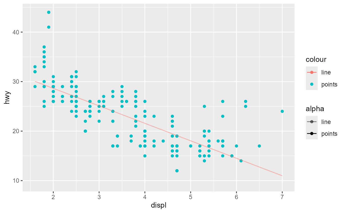
A scatterplot with trendline showing engine displacement versus highway miles per gallon. There are two legends for colour and alpha. Both legends show points and lines separately.

To revert back to the old behaviour, you can set the show.legend = TRUE option in the layers. Like before, the show.legend argument can still be set in an aesthetic-specific way. Setting it to TRUE means ‘always show’, FALSE means ‘never show’ and NA means ‘show if found’.

p +
  geom_point(
    aes(colour = "points", alpha = "points"),
    show.legend = TRUE # always show
  ) +
  geom_line(
    aes(colour = "line", alpha = "line"),
    stat = "smooth", formula = y ~ x, method = "lm",
    show.legend = c(colour = NA, alpha = TRUE) # always show in alpha
  )

The same plot as before, but every legend keys displays points. Lines are shown in every 'alpha' legend key, but only one 'colour' key.

Placement

Legend positions are no longer restricted to just a single side of the plot. By setting the position argument of guides, you can tailor which guides appear where in the plot. Guides that do not have a position set, like the ‘drv’ shape legend below, follow the global theme’s legend.position setting. If we suspend our belief in good data visualisation practice, we can showcase this as follows:

p <- ggplot(mpg, aes(displ, hwy, shape = drv, colour = cty, size = year)) +
  geom_point(aes(alpha = cyl)) +
  guides(
    colour = guide_colourbar(position = "bottom"),
    size   = guide_legend(position = "top"),
    alpha  = guide_legend(position = "inside")
  ) +
  theme(legend.position = "left")
p

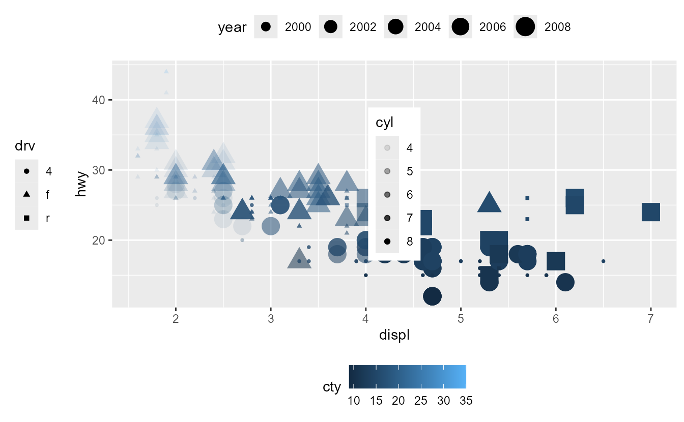
A scatterplot showing engine displacement versus highway miles per gallon. It has four legend placed at the top, left, bottom of the panel and one inside the panel.

In the plot above, the legend for the ‘cyl’ variable is in the middle of the plot. In previous versions of ggplot2, you could set the legend.position to a coordinate to control the placement. However, doing this would change the default legend position, which is not always desirable. To cover such cases, there is now a specialised legend.position.inside argument that controls the positioning of legends with position = "inside" regardless of whether the position was specified in the theme or in the guide.

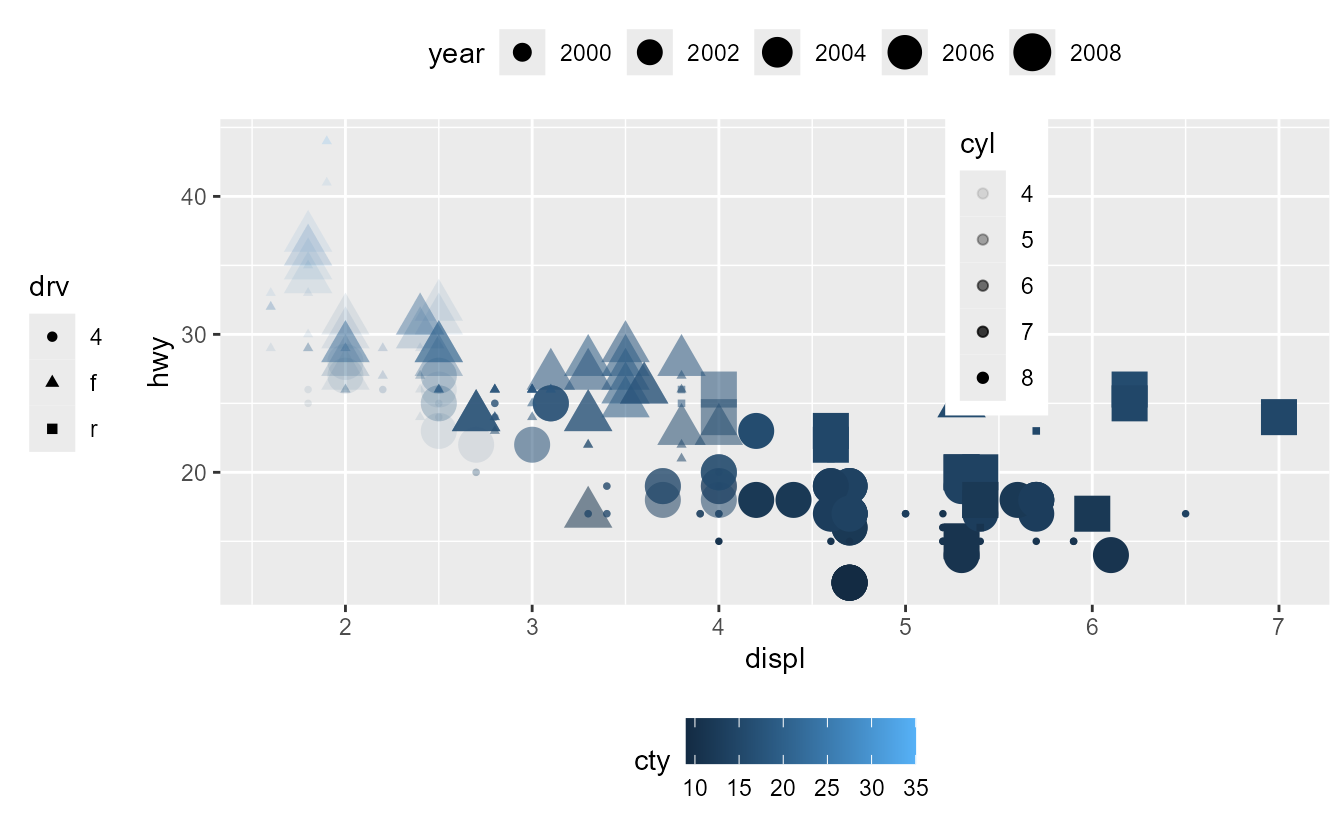
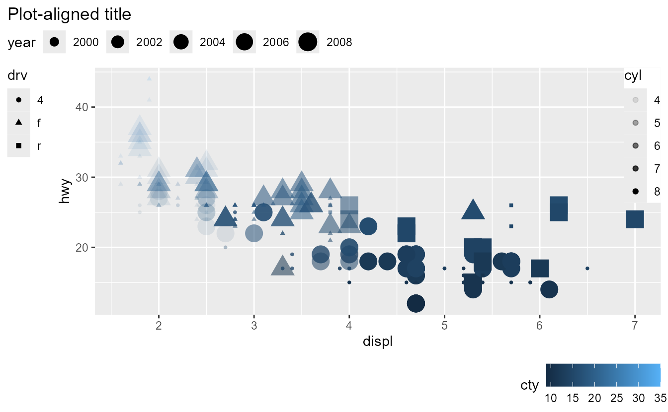
p + theme(legend.position.inside = c(0.7, 0.7))

The same plot as before, but the legend for the 'cyl' variable is to the top-right of the centre.

The justification of legends is controllable by using the legend.justification.{position} theme setting. Moreover, the top and bottom guides can be aligned to the plot rather than the panel by setting the legend.location argument. The main reason behind this is that you can then align the legends with the plot’s title. By default, when plot.title.position = "plot", left legends are already aligned. For this reason, the top and bottom guides are prioritised for the legend.location setting. Moreover, it avoids overlapping of legends in the corners if the justifications would dictate it.

p + 
  labs(title = "Plot-aligned title") +
  theme(
    legend.margin = margin(0, 0, 0, 0), # turned off for alignment
    legend.justification.top = "left",
    legend.justification.left = "top",
    legend.justification.bottom = "right",
    legend.justification.inside = c(1, 1),
    legend.location = "plot",
    plot.title.position = "plot"
  )

The same plot as before, but with a plot-aligned title and different alignments of the legends. The left and top legends are left-aligned with the title.

Spacing and margins

In this release, the way spacing in legends work has been reworked.

The legend.spacing{.x/.y} theme setting is now used to space different guides apart. Previously, it was also used to space legend keys apart; that is no longer the case.
Spacing legend key-label pairs apart is now controlled by the legend.key.spacing{.x/.y} theme setting.
Spacing the labels from the keys is now controlled by the label element’s margin argument.

Because the legend spacing and margin options can be a bit bewildering, a small overview is added below. One setting not included in the overview is legend.spacing.x, which only applies when legend.box = "horizontal". Which exact text margin is relevant for spacing apart keys and labels, or titles and the rest of the guide, depends on the legend.text.position and legend.title.position theme elements.

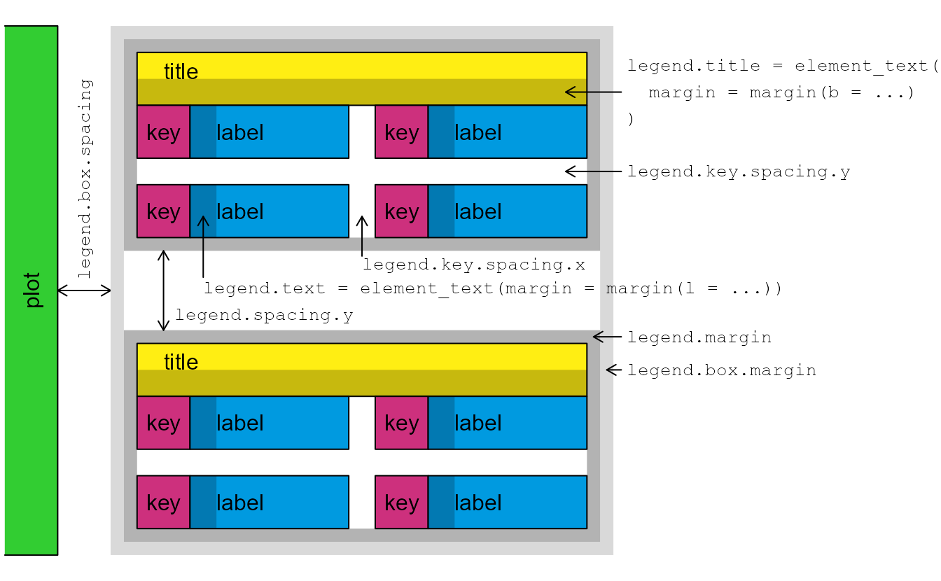
Overview of legend spacing and margin options. Two abstract legends are placed above one another to the right of an area called 'plot'. Various arrows with labels point out different theme settings.

When the titles and keys don’t have explicit margins, appropriate margins are added automatically depending on the text or title position. However, if you override the margins, they will be interpreted literally.

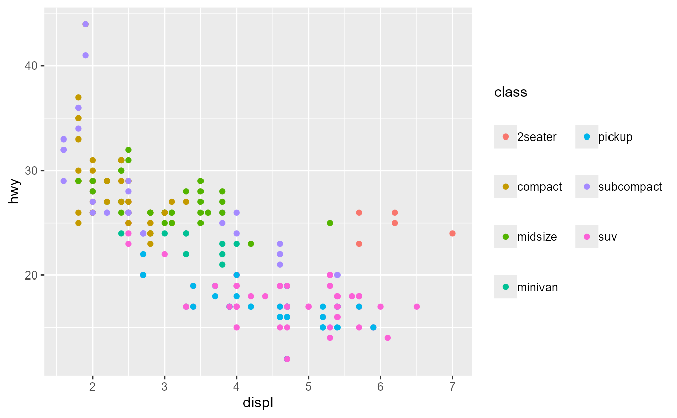
ggplot(mpg, aes(displ, hwy, colour = class)) +
  geom_point() +
  guides(colour = guide_legend(ncol = 2)) +
  theme(
    legend.key.spacing.x = unit(10, "pt"),
    legend.key.spacing.y = unit(20, "pt"),
    legend.text = element_text(margin = margin(l = 0)),
    legend.title = element_text(margin = margin(b = 20))
  )

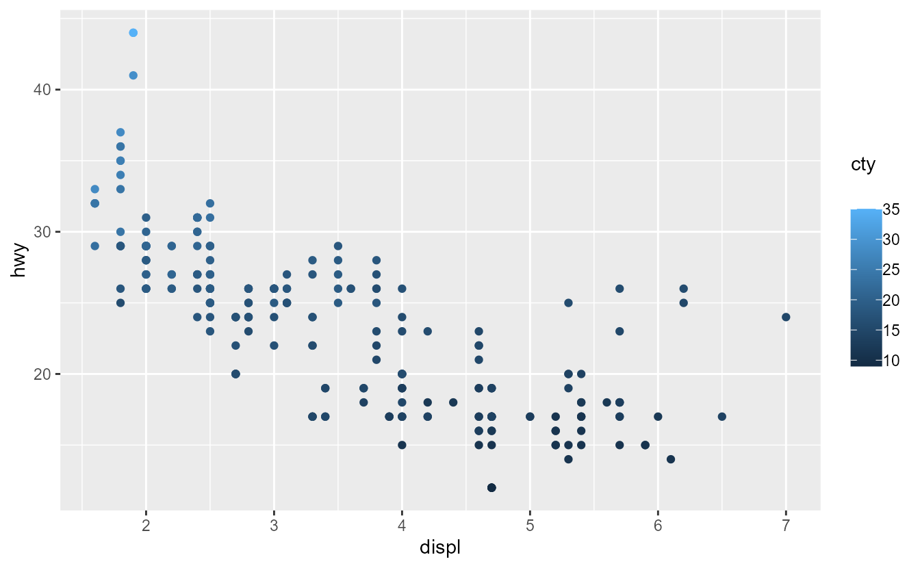
A scatterplot showing engine displacement versus highway miles per gallon. The legend for the 'class' variable shows a key layout with two columns. Keys are widely spacing in the vertical direction and more narrowly in the horizontal direction. There is no space between the keys and their labels, but plenty of space between the legend and its title.

For all intents and purposes, colour bar/step and bins guides are treated as legend guides with just a single key-label pair. While the legend.key.spacing setting does not apply due to it being one single key, the other spacings and margins do apply equally.

ggplot(mpg, aes(displ, hwy, colour = cty)) +
  geom_point() +
  theme(
    legend.text  = element_text(margin = margin(l = 0)),
    legend.title = element_text(margin = margin(b = 20))
  )

The same plot as before, but with a colourbar indicating the 'cty' variable. Again, there is no space between the bar and the labels and ample space between the bar and the title.

Stretching

Another experimental tweak to legends is that they can now have stretching keys (or bars). The option is still considered ‘experimental’ because there are some things that may go wrong. By setting the legend.key{.height/.width} theme argument as a "null" unit, legends can now expand to fill the available space.

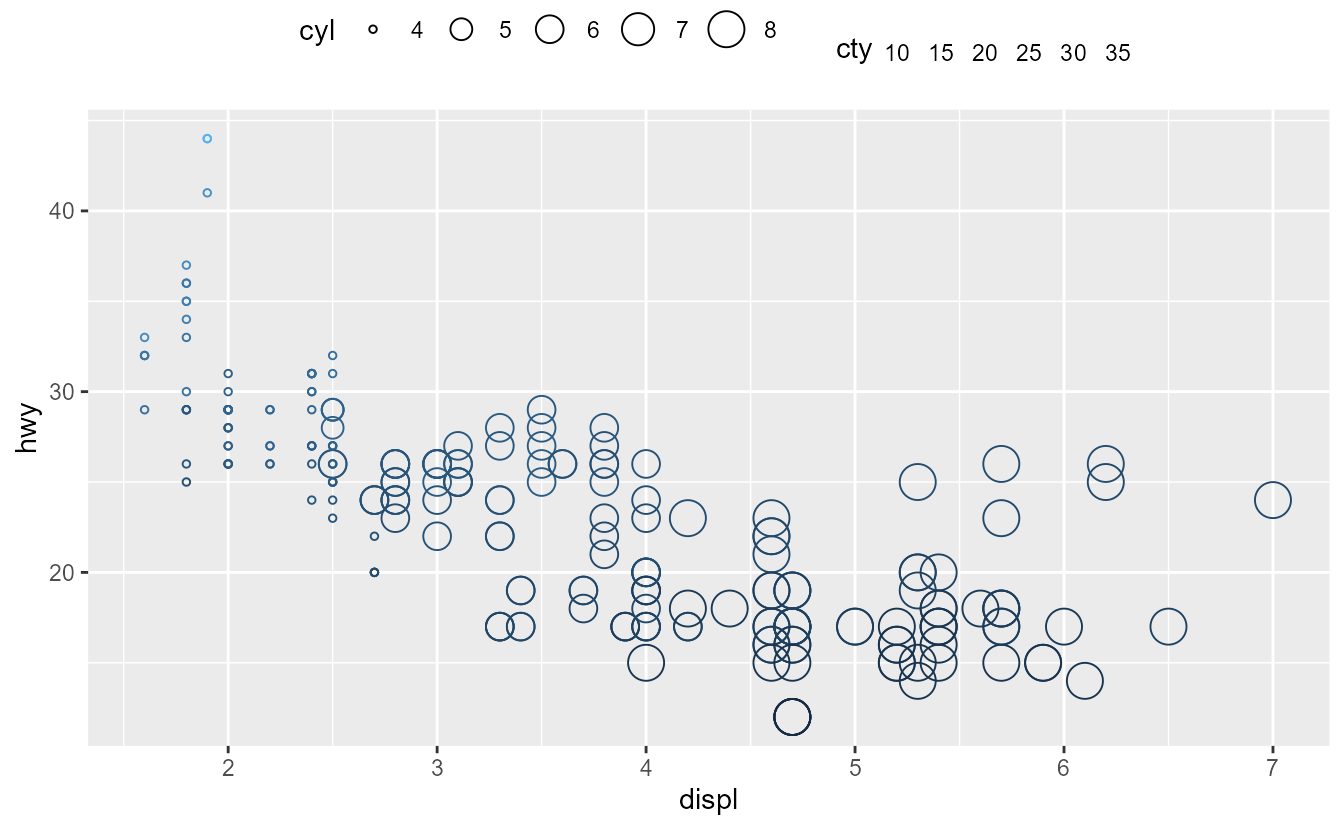
p <- ggplot(mpg, aes(displ, hwy)) +
  geom_point(aes(colour = cty, size = cyl), shape = 21) +
  theme(legend.key.height = unit(1, "null"))
p

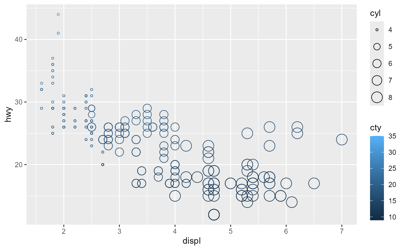
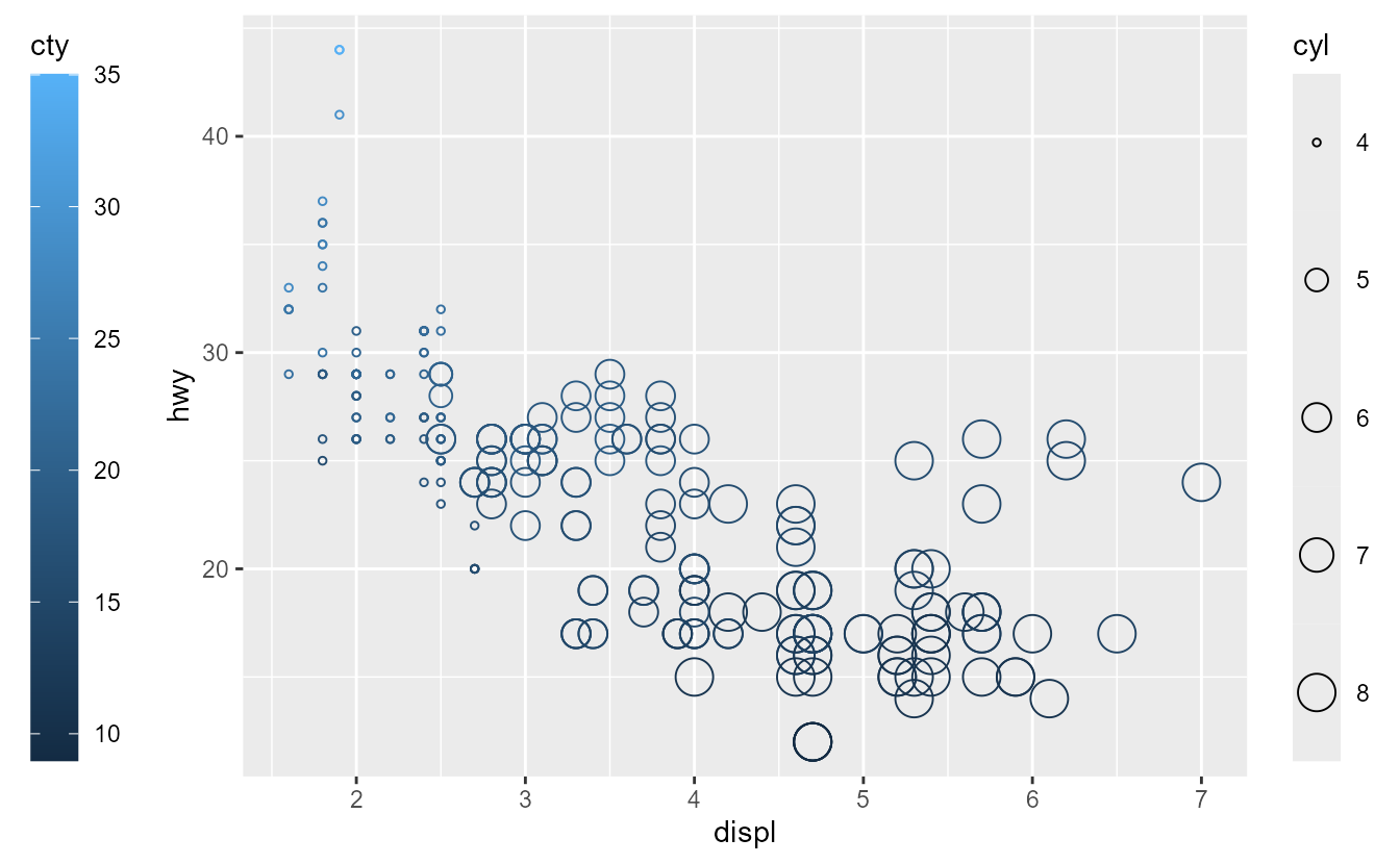
Scatterplot of engine displacement versus highway miles per gallon. There is a legend guide showing the point's size and a colour. Both the legend and the bar take up an approximately equal amount of space on the right-hand side of the panel.

The term ‘available space’ is a tricky one. For starters, other legends placed in the same position take up space, as can be seen in the plot above. If your legend is the only legend in a position, more space is available and it stretches more. As you can see in the plot below, the legends are not aligned with the panel even when stretched. This is because the titles, margins and various spacings all take up space that is not available to stretch into.

p + guides(colour = guide_colourbar(position = "left"))

Same plot as before, but the colour bar is placed on the left. Both the colour bar and legend take up a lot of vertical space.

On the other hand, if one position is packed with legends, the keys may shrink instead of stretch. The keys can become too small to show the aesthetics properly. You can see in the example below that the size legend becomes cut-off due to small keys and text is spaced too closely to comfortably read.

p + aes(fill = model)

Same plot as before, but all legends are on the right, including a new legend for the 'model' variable. All legends have keys that are too small to read the text comfortably, and the points indicating size are clipped.

Another issue that may come up is that the ‘available space’ might be 0. Because the plot itself is also space-filling, setting null-heights for top/bottom positions or null-widths for left/right positions means there is no available space. This may result in the keys or bars becoming invisible. For the plot below, recall that we’ve set the legend.key.height setting to a null unit.

p + theme(legend.position = "top")

Still the same scatterplot but without the fill variable. Legends are placed at the top of the panel, but the bar and key backgrounds have disappeared. The text labels are still present.

Other improvements

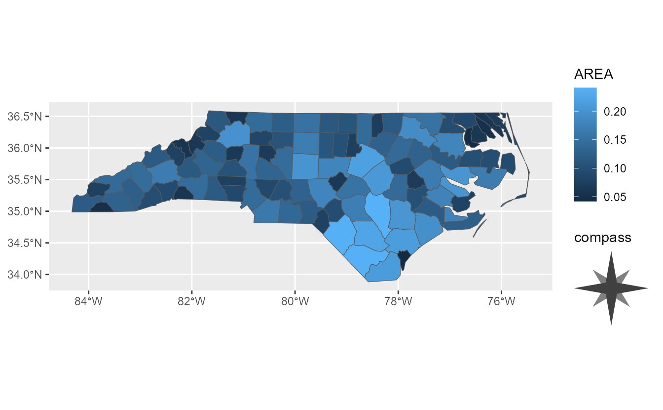
We welcome a new type of legend: guide_custom(). It can be used to add any graphical object (grob) to a plot, like annotation_custom(). There are a few differences though: it is positioned just like a legend and adds titles and margins. In some sense, this guide is ‘special’, as it is the only guide that does not directly reflect a scale. The downside is that it cannot read properties from the plot, but the upside is that it is very flexible. Be careful when your grob does not have an absolute size, you should set the width and height arguments.

x <- c(0.5, 1, 1.5, 1.2, 1.5, 1, 0.5, 0.8, 1, 1.15, 2, 1.15, 1, 0.85, 0, 0.85)
y <- c(1.5, 1.2, 1.5, 1, 0.5, 0.8, 0.5, 1, 2, 1.15, 1, 0.85, 0, 0.85, 1, 1.15)

compass_rose <- grid::polygonGrob(
  x = unit(x, "cm"), y = unit(y, "cm"), id.lengths = c(8, 8),
  gp = grid::gpar(fill = c("grey50", "grey25"), col = NA)
)

nc <- sf::st_read(system.file("shape/nc.shp", package = "sf"), quiet = TRUE)
ggplot(nc) +
  geom_sf(aes(fill = AREA)) +
  guides(custom = guide_custom(compass_rose, title = "compass"))

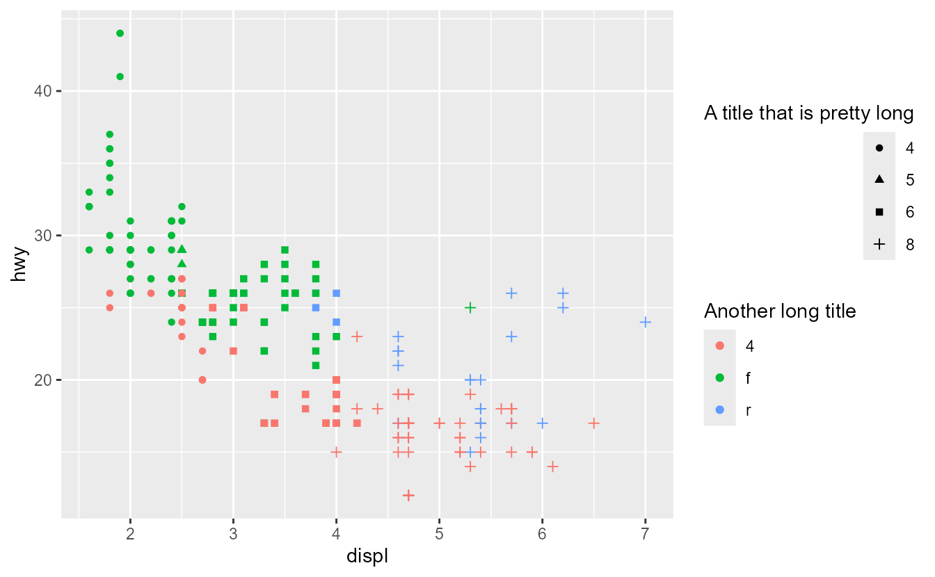
A map of the US state North Carolina, where fill colour indicates the area of counties. Underneath the colour bar for the fill, there is an eight-pointed star to the right of the panel with the title 'compass'.

In previous version of ggplot2, when legend titles are wider than the legends, the guide-title alignment was always left aligned. Now, the justification setting of the legend text determines the alignment: 1 is right or top aligned and 0 is left or bottom aligned.

ggplot(mpg, aes(displ, hwy, shape = factor(cyl), colour = drv)) +
  geom_point() +
  guides(
    shape = guide_legend(
      title = "A title that is pretty long",
      theme = theme(legend.title = element_text(hjust = 1)),
      order = 1
    ),
    colour = guide_legend(
      title = "Another long title",
      theme = theme(legend.title = element_text(hjust = 0))
    )
  )

Scatterplot of engine displacement versus highway miles per gallon. The 'drv' variable has a legend that is left aligned, whereas the 'cyl' variable has a legend that is right-aligned.