
The tidyverse packages provide safe, powerful, and expressive interfaces to solve data science problems. Behind the scenes of the tidyverse is a set of lower-level tools that its developers use to build these interfaces. While these lower-level approaches are more performant than their tidy analogues, their interfaces are often less readable and safe. For most use cases in interactive data analysis, the advantages of tidyverse interfaces far outweigh the drawback in computational speed. When speed becomes an issue, though, transitioning tidy code to use these lower-level interfaces in their backend can offer substantial increases in computational performance.
This post will outline alternatives to tools I love from packages like dplyr and tidyr that I use to speed up computational bottlenecks. These recommendations come from my experiences developing the tidymodels packages, a collection of packages for modeling and machine learning using tidyverse principles. As such, most of these suggestions are best suited to package code, as the noted trade-off is more likely to be worth it in those settings—however, there may also be cases in analytical code, especially in production and/or with very large data sets, where these tips will be helpful. I’ve included a number of “worked examples” with each proposed alternative, showing how the tidymodels team has used these same tricks to speed up our code quite a bit. Before I do that, though, let’s make friends with some new R packages.
Tools of the trade
First, loading the tidyverse:
The most important tools to help you understand what’s slowing your code down have little to do with the tidyverse at all!
profvis
The profvis package is an R package for collecting and visualizing profiling data.
Profiling is the process of determining how long different portions of a chunk of code take to run. For example, in this next function slow_function(), it’s somewhat straightforward to tell how long different portions of the following code run for if you know what
pause() does. (
pause() is a function from the profvis package that just chills out for the specified amount of time. For example, pause(1) will wait for 1 second before finishing running.)
step_1 <- function() {
  pause(1)
}

step_2 <- function() {
  pause(2)
}

slow_function <- function() {
  step_1()

  step_2()

  TRUE
}
Profiling tools would help us see that step_1() takes one second, while step_2() takes two. In practice, this is usually much harder to intuit visually. To profile code with profvis, use the
profvis() function:
result <- profvis(slow_function())Printing the resulting object out will visualize the time different calls within slow_function() took:
result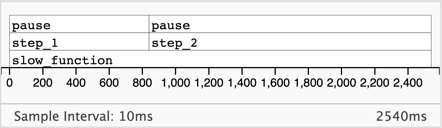
This output shows that, inside of slow_function(), step_1() took about a third of the total time and step_2() took two-thirds. All of the time in both of those functions was due to calling
pause().
Profiling should be your first line of defense against slow-running code. Often, profiling will surface slowdowns in unexpected places, and solutions to address those slowdowns may have little to do with usage of tidy tools. To learn more about profiling, the Measuring performance chapter in Hadley Wickham’s book Advanced R is a great place to start.
bench
profvis is a powerful tool to surface code slowdowns. Often, though, it may not be immediately clear how to fix that slowdown. The bench package allows users to quickly test out how long different approaches to solving a problem take.
For example, say we want to take the sum of the numbers in a list, but we’ve identified via profiling that this operation is slowing our code down:
numbers <- as.list(1:5)

numbers
#> [[1]]
#> [1] 1
#>
#> [[2]]
#> [1] 2
#>
#> [[3]]
#> [1] 3
#>
#> [[4]]
#> [1] 4
#>
#> [[5]]
#> [1] 5
One approach could be using the
Reduce() function:
Reduce(sum, numbers)
#> [1] 15
Another could involve converting to a vector with
unlist() and then using
sum():
You may have some other ideas of how to solve this problem! How do we figure out which one is fastest, though? The
bench::mark() function from bench takes in different proposals to solve the same problem and returns a tibble with information about how long they took (among other things.)
res <-
  bench::mark(
    approach_1 = Reduce(sum, numbers),
    approach_2 = sum(unlist(numbers))
  )

res %>% select(expression, median)
#> # A tibble: 2 × 2
#>   expression   median
#>   <bch:expr> <bch:tm>
#> 1 approach_1   2.25µs
#> 2 approach_2 491.97ns
The other nice part about
bench::mark() is that it will check that each approach gives the same output, so that you don’t mistakenly compare apples and oranges.
There are two important lessons to take in from this output:
- The
sum(unlist())approach was wicked fast compared toReduce(). - Both of these expressions were fast. Even the slower of the two took 2.25µs—to put that in perspective, that expression could complete 443454 iterations in a second! Keeping this bigger picture in mind is always important when benchmarking; if code runs fast enough to not be an issue in practical situations, then it need not be optimized in favor of less readable or safe code.
The results of little experiments like this one can be surprising at first. Over time, though, you will develop intuition for the fastest way to solve problems you commonly solve, and will write fast code the first time around!
In this case, using
Reduce() means calling
sum() many times, approximately once for each element of the list, and while
sum() isn’t particularly slow, calling an R function many times tends to have non-negligible overhead. With the sum(unlist()) approach, there are only 2 R function calls—one for
unlist() and one for
sum()—which both immediately drop into C code.
vctrs
The problems I commonly solve—and possibly you as well, as a reader of this post—often involve lots of dplyr and tidyr. When profiling the tidymodels packages, I’ve come across many places where calls to dplyr and tidyr took more time than I’d like them to, but had a lot to learn about how to speed up those operations. Enter the vctrs package!
If you use dplyr and tidyr like I do, turns out you’re also a vctrs user! dplyr and tidyr rely on vctrs to handle all sorts of elementary operations behind the scenes, and the package is a core part of a tidy developer’s toolkit. Taken together with some functions from the tibble package, these tools provide a super efficient, albeit bare-bones, alternative interface to common data manipulation tasks like
filter()ing and
select()ing.
Rewriting tidy code
For every performance improvement I make by rewriting dplyr and tidyr code to instead use vctrs and tibble, I make probably two or three simpler optimizations. Tool-agnostic practices such as reducing duplicated computations, implementing early returns where possible, and using vectorized implementations will likely take you far when optimizing R code. Profiling is your ground truth! When profiling indicates that otherwise well-factored code is slowed by tidy interfaces, though, all is not lost.
We’ll demonstrate different ways to speed up tidy code using a version of the base R data frame mtcars converted to a tibble:
mtcars_tbl <- as_tibble(mtcars, rownames = "make_model")

mtcars_tbl
#> # A tibble: 32 × 12
#>    make_model    mpg   cyl  disp    hp  drat    wt  qsec    vs    am  gear  carb
#>    <chr>       <dbl> <dbl> <dbl> <dbl> <dbl> <dbl> <dbl> <dbl> <dbl> <dbl> <dbl>
#>  1 Mazda RX4    21       6  160    110  3.9   2.62  16.5     0     1     4     4
#>  2 Mazda RX4 …  21       6  160    110  3.9   2.88  17.0     0     1     4     4
#>  3 Datsun 710   22.8     4  108     93  3.85  2.32  18.6     1     1     4     1
#>  4 Hornet 4 D…  21.4     6  258    110  3.08  3.22  19.4     1     0     3     1
#>  5 Hornet Spo…  18.7     8  360    175  3.15  3.44  17.0     0     0     3     2
#>  6 Valiant      18.1     6  225    105  2.76  3.46  20.2     1     0     3     1
#>  7 Duster 360   14.3     8  360    245  3.21  3.57  15.8     0     0     3     4
#>  8 Merc 240D    24.4     4  147.    62  3.69  3.19  20       1     0     4     2
#>  9 Merc 230     22.8     4  141.    95  3.92  3.15  22.9     1     0     4     2
#> 10 Merc 280     19.2     6  168.   123  3.92  3.44  18.3     1     0     4     4
#> # ℹ 22 more rows
One-for-one replacements
Many of the core functions in dplyr have alternatives in vctrs and tibble that can be quickly transitioned. There are a couple considerations associated with each, though, and some of them make piping a bit more awkward—most of the time, when I switch these out, I remove the pipe %>% as well.
filter()
The dplyr code:
…can be replaced by:
vec_slice(mtcars_tbl, mtcars_tbl$hp > 100)Note that the second argument that determines which rows to keep requires you to actually pass the column mtcars_tbl$hp rather than its reference hp. If you feel cozier with square brackets, you can also use [.tbl_df:
mtcars_tbl[mtcars_tbl$hp > 100, ][.tbl_df is the
method for subsetting with a single square bracket when applied to tibbles. Tibbles have their own methods for extracting and replacing subsets of data frames. They generally behave similarly to the analogous methods for data.frames, but have small differences to improve consistency and safety.
The benchmarks for these different approaches are:
res <-
  bench::mark(
    dplyr = filter(mtcars_tbl, hp > 100),
    vctrs = vec_slice(mtcars_tbl, mtcars_tbl$hp > 100),
    `[.tbl_df` = mtcars_tbl[mtcars_tbl$hp > 100, ]
  ) %>%
    select(expression, median)

res
#> # A tibble: 3 × 2
#>   expression   median
#>   <bch:expr> <bch:tm>
#> 1 dplyr      289.93µs
#> 2 vctrs        4.63µs
#> 3 [.tbl_df    23.74µs
The bigger picture of benchmarking is worth re-iterating here. While the filter() approach was by far the slowest expression of the three, it still only took 290µs—able to complete 3449 iterations in a second. If I’m interactively analyzing data, I won’t even notice the difference in evaluation time between these expressions, let alone care about it; the benefits of expressiveness and safety that filter() provide far outweigh the drawback of this slowdown. If filter() is called 3449 times in the backend of a machine learning pipeline, though, these alternatives may be worth transitioning to.
Some examples of changes like this made to tidymodels packages: tidymodels/parsnip#935, tidymodels/parsnip#933, tidymodels/parsnip#901.
mutate()
The dplyr code:
mtcars_tbl <- mutate(mtcars_tbl, year = 1974L)…can be replaced by:
mtcars_tbl$year <- 1974L…with benchmarks:
bench::mark(
  dplyr = mutate(mtcars_tbl, year = 1974L),
  `$<-.tbl_df` = {mtcars_tbl$year <- 1974L; mtcars_tbl}
) %>%
  select(expression, median)
#> # A tibble: 2 × 2
#>   expression   median
#>   <bch:expr> <bch:tm>
#> 1 dplyr       302.5µs
#> 2 $<-.tbl_df   12.8µs
By default, both mutate() and $<-.tbl_df append the new column at the right-most position. The .before and .after arguments to mutate() are a really nice interface to adjust that behavior, and I miss it often when using $<-.tbl_df. In those cases, select() and its alternatives (see next section!) can be helpful.
Some examples of changes like this made to tidymodels packages: tidymodels/parsnip#933, tidymodels/parsnip#921, and tidymodels/parsnip#901.
select()
The dplyr code:
select(mtcars_tbl, hp)…can be replaced by:
mtcars_tbl["hp"]…with benchmarks:
bench::mark(
  dplyr = select(mtcars_tbl, hp),
  `[.tbl_df` = mtcars_tbl["hp"]
) %>%
  select(expression, median)
#> # A tibble: 2 × 2
#>   expression   median
#>   <bch:expr> <bch:tm>
#> 1 dplyr      527.01µs
#> 2 [.tbl_df     8.08µs
Of course, the nice part about select(), and something we make use of in tidymodels quite a bit, is tidyselect. I’ve often found that we lean heavily on selecting via external vectors, i.e. character vectors, i.e. things that can be inputted to [.tbl_df directly. That is:
cols <- c("hp", "wt")

bench::mark(
  dplyr = select(mtcars_tbl, all_of(cols)),
  `[.tbl_df` = mtcars_tbl[cols]
) %>%
  select(expression, median)
#> # A tibble: 2 × 2
#>   expression   median
#>   <bch:expr> <bch:tm>
#> 1 dplyr      548.74µs
#> 2 [.tbl_df     8.53µs
Note that [.tbl_df always sets drop = FALSE.
[.tbl_df can also be used as an alternative interface to select() or relocate() with a .before or .after argument. For instance, to place that column year we made in the last section as the second column, we could write:
left_cols <- c("make_model", "year")

mtcars_tbl[
  c(left_cols,
    setdiff(colnames(mtcars_tbl), left_cols)
  )
]
No, thanks, but it is a good bit faster than tidyselect-based alternatives:
bench::mark(
  mutate = mutate(mtcars_tbl, year = 1974L, .after = make_model),
  relocate = relocate(mtcars_tbl, year, .after = make_model),
  `[.tbl_df` =
      mtcars_tbl[
        c(left_cols,
          colnames(mtcars_tbl[!colnames(mtcars_tbl) %in% left_cols])
        )
      ],
  check = FALSE
) %>%
  select(expression, median)
#> # A tibble: 3 × 2
#>   expression   median
#>   <bch:expr> <bch:tm>
#> 1 mutate        1.2ms
#> 2 relocate    804.3µs
#> 3 [.tbl_df     19.1µs
Some examples of changes like this made to tidymodels packages: tidymodels/parsnip#935, tidymodels/parsnip#933, tidymodels/parsnip#921, and tidymodels/tune#635.
pull()
The dplyr code:
pull(mtcars_tbl, hp)…can be replaced by:
mtcars_tbl$hp…or:
mtcars_tbl[["hp"]]Note that, for tibbles, $ will raise a warning if the subsetted column doesn’t exist, while [[ will silently return NULL.
With benchmarks:
bench::mark(
  dplyr = pull(mtcars_tbl, hp),
  `$.tbl_df` = mtcars_tbl$hp,
  `[[.tbl_df` = mtcars_tbl[["hp"]]
) %>%
  select(expression, median)
#> # A tibble: 3 × 2
#>   expression   median
#>   <bch:expr> <bch:tm>
#> 1 dplyr      101.19µs
#> 2 $.tbl_df   615.02ns
#> 3 [[.tbl_df    2.25µs
Some examples of changes like this made to tidymodels packages: tidymodels/parsnip#935 and tidymodels/tune#635.
bind_*()
bind_rows() and bind_cols() can be substituted for vec_rbind() and vec_cbind(), respectively. First, row-binding:
bench::mark(
  dplyr = bind_rows(mtcars_tbl, mtcars_tbl),
  vctrs = vec_rbind(mtcars_tbl, mtcars_tbl)
) %>%
  select(expression, median)
#> # A tibble: 2 × 2
#>   expression   median
#>   <bch:expr> <bch:tm>
#> 1 dplyr          44µs
#> 2 vctrs        14.3µs
As for column-binding:
tbl <- tibble(year = rep(1974L, nrow(mtcars_tbl)))

bench::mark(
  dplyr = bind_cols(mtcars_tbl, tbl),
  vctrs = vec_cbind(mtcars_tbl, tbl)
) %>%
  select(expression, median)
#> # A tibble: 2 × 2
#>   expression   median
#>   <bch:expr> <bch:tm>
#> 1 dplyr        60.7µs
#> 2 vctrs        26.2µs
Some examples of changes like this made to tidymodels packages: tidymodels/tune#636.
Grouping
In general, the introduction of groups makes these substitutions much trickier. In those cases, it’s likely best to weigh (via profiling) how significant the slowdown is and, if it’s not too bad, opt not to make any changes. For code that relies on group_by() and sees heavy traffic, see vctrs::list_unchop(), vctrs::vec_chop(), and vctrs::vec_rep_each().
Tibbles
Tibbles are great, and I don’t want to interface with any other data frame-y thing. Some notes:
as_tibble()on a tibble is not “free”:bench::mark( on_tbl_df = as_tibble(mtcars_tbl), on_data.frame = as_tibble(mtcars, rownames = "make_model") ) %>% select(expression, median) #> # A tibble: 2 × 2 #> expression median #> <bch:expr> <bch:tm> #> 1 on_tbl_df 51.2µs #> 2 on_data.frame 238.6µsNote that the time to coerce data frames and tibbles doesn’t depend on the size of the data being coerced, in most situations.
Building a tibble from scratch using
tibble()actually takes quite a while as well.tibble()handles vector recycling and name checking, builds columns sequentially, all that good stuff. If you need that, usetibble(), but if you’re building a tibble from well-understood inputs, usenew_tibble(), which minimizes validation checks. For a middle ground betweentibble()andnew_tibble(list())in terms of both performance and safety, use thedf_list()function from the vctrs package in place oflist().bench::mark( tibble = tibble(a = 1:2, b = 3:4), new_tibble_df_list = new_tibble(df_list(a = 1:2, b = 3:4), nrow = 2), new_tibble_list = new_tibble(list(a = 1:2, b = 3:4), nrow = 2) ) %>% select(expression, median) #> # A tibble: 3 × 2 #> expression median #> <bch:expr> <bch:tm> #> 1 tibble 165.97µs #> 2 new_tibble_df_list 16.69µs #> 3 new_tibble_list 4.96µsNote that
new_tibble()will not check the lengths of its inputs. Carry out simple recycling yourself, and be sure to use thenrowargument to get basic length checks.
Some examples of changes like this made to tidymodels packages: tidymodels/parsnip#945, tidymodels/parsnip#934, tidymodels/parsnip#929, tidymodels/parsnip#923, tidymodels/parsnip#902, tidymodels/dials#277, and tidymodels/tune#637.
Becoming join-critical
Two truths:
dplyr joins are a remarkably safe and powerful way to synthesize data sources.
One ought to ask themselves “does this really need to be a join?” when combining data sources in package code.
Some ways to intuit about join efficiency:
If this join happens multiple times, is it possible to express it as one join and then subset it when needed? i.e. if a join happens inside of a loop but the elements of the join are not indices of the loop, it’s likely possible to pull that join outside of the loop and then
vec_slice()its results inside of the loop.Am I using the complete outputted join result or just a portion? If I end up only making use of column names, or values in one column (as with joins approximating lookup tables), or pairings between two columns, I may be able to instead use
$.tbl_dfor[.tbl_df.
As an example, imagine we have another tibble that tells us additional information about the make_models that I’ve driven:
my_cars <-
  tibble(
    make_model = c("Honda Civic", "Subaru Forester"),
    color = c("Grey", "White")
  )

my_cars
#> # A tibble: 2 × 2
#>   make_model      color
#>   <chr>           <chr>
#> 1 Honda Civic     Grey
#> 2 Subaru Forester White
I could use a join to subset down to cars in mtcars_tbl and add this information on the cars I’ve driven:
inner_join(mtcars_tbl, my_cars, "make_model")
#> # A tibble: 1 × 13
#>   make_model    mpg   cyl  disp    hp  drat    wt  qsec    vs    am  gear  carb
#>   <chr>       <dbl> <dbl> <dbl> <dbl> <dbl> <dbl> <dbl> <dbl> <dbl> <dbl> <dbl>
#> 1 Honda Civic  30.4     4  75.7    52  4.93  1.62  18.5     1     1     4     2
#> # ℹ 1 more variable: color <chr>
Another way to express this, though, if I can safely assume that each of my cars would have only one or zero matches in mtcars_tbl, is to find entries in mtcars_tbl$make_model that match entries in my_cars$make_model, subset down to those matches, and then bind columns:
supplement_my_cars <- function() {
  # locate matches, assuming only 0 or 1 matches possible
  loc <- vec_match(my_cars$make_model, mtcars_tbl$make_model)

  # keep only the matches
  loc_mine <- which(!is.na(loc))
  loc_mtcars <- vec_slice(loc, !is.na(loc))

  # drop duplicated join column
  my_cars_join <- my_cars[setdiff(names(my_cars), "make_model")]

  vec_cbind(
    vec_slice(mtcars_tbl, loc_mtcars),
    vec_slice(my_cars_join, loc_mine)
  )
}

supplement_my_cars()
#> # A tibble: 1 × 13
#>   make_model    mpg   cyl  disp    hp  drat    wt  qsec    vs    am  gear  carb
#>   <chr>       <dbl> <dbl> <dbl> <dbl> <dbl> <dbl> <dbl> <dbl> <dbl> <dbl> <dbl>
#> 1 Honda Civic  30.4     4  75.7    52  4.93  1.62  18.5     1     1     4     2
#> # ℹ 1 more variable: color <chr>
This is indeed quite a bit faster:
bench::mark(
  inner_join = inner_join(mtcars_tbl, my_cars, "make_model"),
  manual = supplement_my_cars()
) %>%
  select(expression, median)
#> # A tibble: 2 × 2
#>   expression   median
#>   <bch:expr> <bch:tm>
#> 1 inner_join    438µs
#> 2 manual       50.7µs
At the same time, if either of these problems were even a little bit more complex, e.g. if there were possibly multiple matching make_models in mtcars_tbl or if I wanted to keep all rows in mtcars_tbl regardless of whether I had driven the car, then expressing this join with more bare-bones operations quickly becomes less readable and more error-prone. In those cases, too, joins in dplyr have a relatively small amount of overhead when compared to the vctrs backends underlying them. So, optimize carefully!
Some examples of writing out joins in tidymodels packages: tidymodels/parsnip#932, tidymodels/parsnip#931, tidymodels/parsnip#921, and tidymodels/recipes#1121.
nest()
nest()s are subject to similar considerations as joins. When they allow for expressive or principled user interfaces, use them, but manipulate them sparingly in backends. Writing out nest() calls can result in substantial speedups, though, and the process is not quite as gnarly as writing out a join. For code that relies on nest()s and sees heavy traffic, rewriting with vctrs may be worth the effort.
For example, consider nesting mtcars_tbl by cyl and am:
nest(mtcars_tbl, .by = c(cyl, am))
#> # A tibble: 6 × 3
#>     cyl    am data
#>   <dbl> <dbl> <list>
#> 1     6     1 <tibble [3 × 10]>
#> 2     4     1 <tibble [8 × 10]>
#> 3     6     0 <tibble [4 × 10]>
#> 4     8     0 <tibble [12 × 10]>
#> 5     4     0 <tibble [3 × 10]>
#> 6     8     1 <tibble [2 × 10]>
For some basic nests, vec_split() can do the trick.
nest_cols <- c("cyl", "am")

res <-
  vec_split(
    x = mtcars_tbl[setdiff(colnames(mtcars_tbl), nest_cols)],
    by = mtcars_tbl[nest_cols]
  )

vec_cbind(res$key, new_tibble(list(data = res$val)))
#> # A tibble: 6 × 3
#>     cyl    am data
#>   <dbl> <dbl> <list>
#> 1     6     1 <tibble [3 × 10]>
#> 2     4     1 <tibble [8 × 10]>
#> 3     6     0 <tibble [4 × 10]>
#> 4     8     0 <tibble [12 × 10]>
#> 5     4     0 <tibble [3 × 10]>
#> 6     8     1 <tibble [2 × 10]>
The performance improvement in these situations can be quite substantial:
bench::mark(
  nest = nest(mtcars_tbl, .by = c(cyl, am)),
  vctrs = {
    res <-
      vec_split(
        x = mtcars_tbl[setdiff(colnames(mtcars_tbl), nest_cols)],
        by = mtcars_tbl[nest_cols]
      )

    vec_cbind(res$key, new_tibble(list(data = res$val)))
  }
) %>%
  select(expression, median)
#> # A tibble: 2 × 2
#>   expression   median
#>   <bch:expr> <bch:tm>
#> 1 nest         1.81ms
#> 2 vctrs       67.61µs
More complex nests require a good bit of facility with the vctrs package. vec_split(), list_unchop(), and vec_chop() are all good places to start, and these examples of writing out nests in tidymodels packages make use of other vctrs patterns:
tidymodels/tune#657,
tidymodels/tune#657,
tidymodels/tune#640, and
tidymodels/recipes#1121.
Combining strings
The glue package is super helpful for writing expressive and correct strings with data, though it is quite a bit slower than paste0(). At the same time, paste0() has some tricky recycling behavior. For a middle ground in terms of both performance and safety, this short wrapper has been quite helpful:
vec_paste0 <- function (...) {
  args <- vec_recycle_common(...)
  exec(paste0, !!!args)
}
name <- "Simon"
bench::mark(
glue = glue::glue("My name is {name}."),
vec_paste0 = vec_paste0("My name is ", name, "."),
paste0 = paste0("My name is ", name, "."),
check = FALSE
) %>%
select(expression, median)
#> # A tibble: 3 × 2
#> expression median
#> <bch:expr> <bch:tm>
#> 1 glue 38.99µs
#> 2 vec_paste0 3.98µs
#> 3 paste0 861.01ns
My rule of thumb is to use glue() for errors, when the function will stop executing anyway. For simple pastes that are intended to be called repeatedly, use vec_paste0(). There’s a lot of gray area in between those two contexts—intuit (or profile) as you will.
Wrapping up
This post contains a number of tricks that offer especially performant alternatives to interfaces from dplyr and tidyr. Making use of these backend tools is certainly a trade-off; what is gained in computational performance is also offset by a decline in readability and safety, so developers ought to consider carefully when optimizations are worth the effort and risk.
Thanks to Davis Vaughan for the guidance in getting started with vctrs. Also, thanks to both Davis Vaughan and Lionel Henry for their efforts in helping the tidymodels team address the bottlenecks that have been surfaced by our work on optimizations in tidyverse packages.