
Meet the map() family
purrr’s
map() family of functions are tools for iteration, performing the same action on multiple inputs. If you’re new to purrr, the
Iteration chapter of R for Data Science is a good place to get started.
One of the benefits of using
map() is that the function has variants (e.g.
map2(),
pmap(), etc.) all of which work the same way. To borrow from Jennifer Thompson’s excellent
Intro to purrr,the arguments can be broken into two groups: what we’re iterating over, and what we’re doing each time. The adapted figure below shows what this looks like for
map(),
map2(), and
pmap().
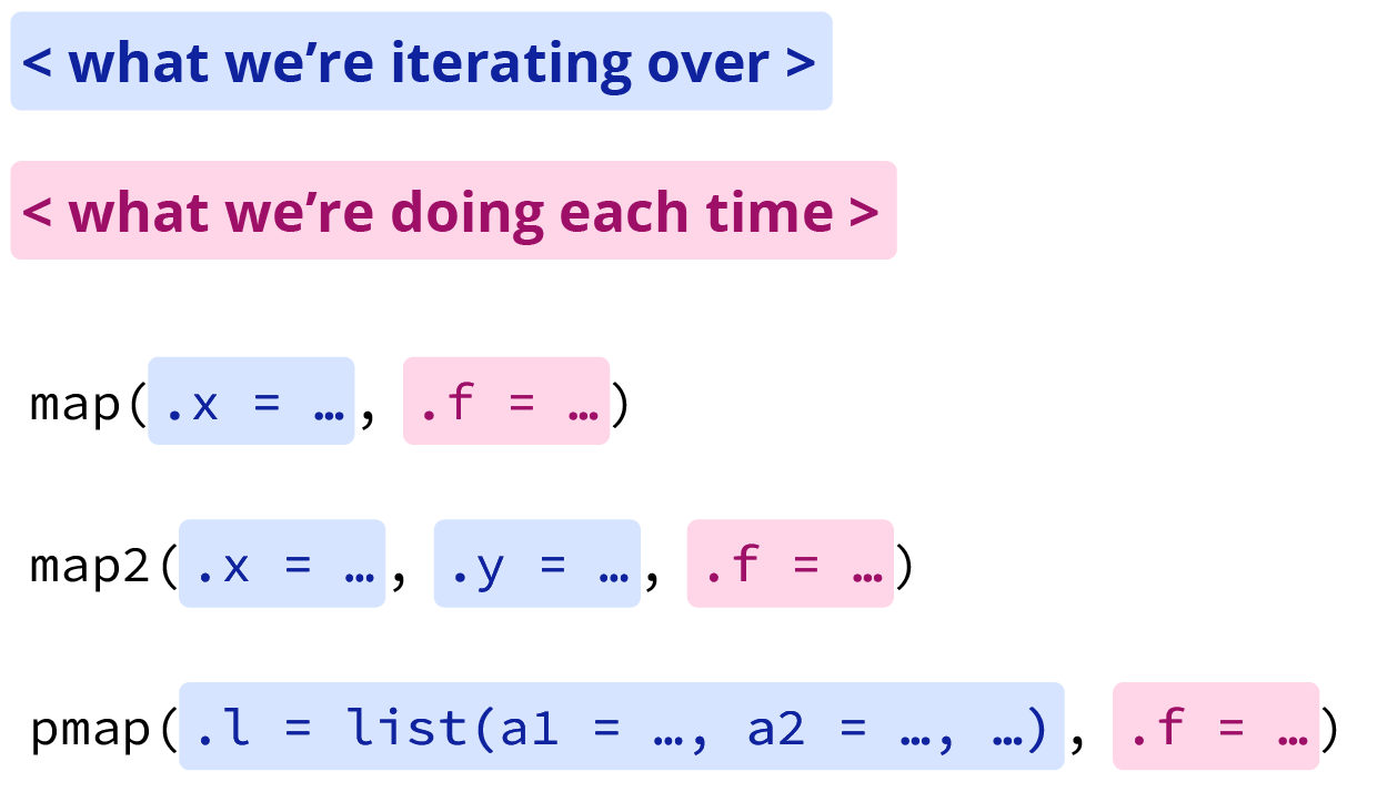
Grouped map function arguments, adapted from Intro to purrr by Jennifer Thompson
In addition to handling different input arguments, the map family of functions has variants that create different outputs. The following table from the Map-variants section of Advanced R shows how the orthogonal inputs and outputs can be used to organise the variants into a matrix:
| List | Atomic | Same type | Nothing | |
|---|---|---|---|---|
| One argument | map() | map_lgl(), … | modify() | walk() |
| Two arguments | map2() | map2_lgl(), … | modify2() | walk2() |
| One argument + index | imap() | imap_lgl(), … | imodify() | iwalk() |
| N arguments | pmap() | pmap_lgl(), … | — | pwalk() |
What’s up with walk()?
Based on the table above, you might think that
walk() isn’t very useful. Indeed,
walk(),
walk2(), and
pwalk() all invisibly return .x. However, they come in handy when you want to call a function for its side effects rather than its return value.
Here, we’ll go through two common use cases: saving multiple CSVs, and multiple plots. We’ll also make use of the fs package, a cross-platform interface to file system operations, to inspect our outputs.
If you want to try this out but don’t want to save files locally, there’s a companion project on Posit Cloud where you can follow along.
Writing (and deleting) multiple CSVs
To get started, we’ll need some data. Let’s use the
gapminder example Sheet built into
googlesheets4. Because there are multiple worksheets (one for each continent), we’ll use
map() to apply
read_sheet()1 to each one, and get back a list of data frames.
ss <- gs4_example("gapminder") # get sheet id
sheets <- sheet_names(ss) # get the names of individual sheets
gap_dfs <- map(sheets, .f = \(x) read_sheet(ss, sheet = x))
#> ✔ Reading from gapminder.
#> ✔ Range ''Africa''.
#> ✔ Reading from gapminder.
#> ✔ Range ''Americas''.
#> ✔ Reading from gapminder.
#> ✔ Range ''Asia''.
#> ✔ Reading from gapminder.
#> ✔ Range ''Europe''.
#> ✔ Reading from gapminder.
#> ✔ Range ''Oceania''.
Note that the backslash syntax for anonymous functions (e.g. \(x) x + 1) was introduced in base R version 4.1.0 as a shorthand for function(x) x + 1. If you’re using an earlier version of R, you can use purrr’s shorthand: a formula (e.g. ~ .x + 1).
Typically, you’d want to combine these data frames into one to make it easier to work with your data. To do so, we’ll use
list_rbind() on gap_dfs. I’ve kept the intermediary object, since we’ll use it in a moment with
walk(), but could have just as easily piped the output directly. The combination of
purrr::map() and
list_rbind() is a handy one that you can learn more about in the
R for Data Science.
gap_combined <- gap_dfs |>
  list_rbind()
Now let’s say that, for whatever reason, you’d like to save the data from these sheets as individual CSVs. This is where
walk() comes into play—writing out the file with
write_csv() is a “side effect.” We’ll use
fs::dir_create() to create a data folder to put our files into2, and build a vector of paths/file names. Since we have two arguments, the list of data frames, and the paths, we’ll use
walk2().
fs::dir_create("data")
paths <- str_glue("data/gapminder_{tolower(sheets)}.csv")
walk2(
  gap_dfs,
  paths,
  \(df, name) write_csv(df, name)
  )
To see what we’ve done, we can use
fs::dir_tree() to see the contents of the directory as a tree, or
fs::dir_ls() to return the paths as a vector. These functions also take glob and regexp arguments, allowing you to filter paths by file type with globbing patterns (e.g. *.csv) or using a regular expression passed on to
grep().
fs::dir_tree("data")
#> data
#> ├── gapminder_africa.csv
#> ├── gapminder_americas.csv
#> ├── gapminder_asia.csv
#> ├── gapminder_europe.csv
#> └── gapminder_oceania.csv
fs::dir_ls("data")
#> data/gapminder_africa.csv   data/gapminder_americas.csv
#> data/gapminder_asia.csv     data/gapminder_europe.csv
#> data/gapminder_oceania.csv
If you’re having regrets, or want to return your example project to its previous state, it’s just as easy to
walk()
fs::file_delete() along those same paths.3
walk(paths, \(paths) fs::file_delete(paths))Saving multiple plots
Now, let’s say you want to create and save a bunch of plots. We’ll use a modified version of the
conditional_bars()4 function from the R for Data Science chapter on writing
functions, and the built-in
diamonds dataset.
# modified conditional bars function from R4DS
conditional_bars <- function(df, condition, var) {
df |>
filter({{ condition }}) |>
ggplot(aes(x = {{ var }})) +
geom_bar() +
ggtitle(rlang::englue("Count of diamonds by {{var}} where {{condition}}"))
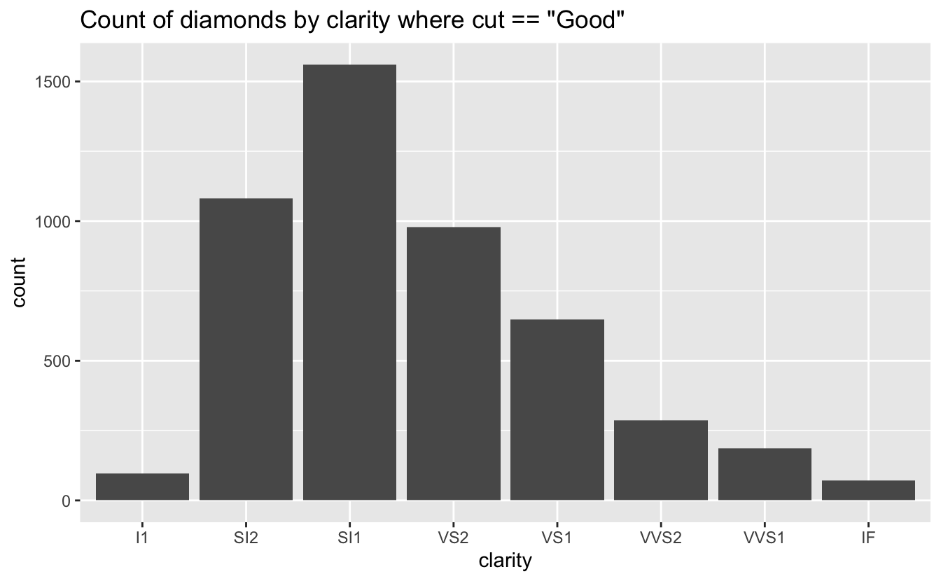
}It’s easy enough to run this for one condition, for example for the diamonds with cut == "Good".
diamonds |> conditional_bars(cut == "Good", clarity)
But what if we want to make and save a plot for each cut? Again, it’s
map() and
walk() to the rescue.
Because we’re using the same data (diamonds) and conditioning on the same variable (cut), we’ll only need to
map() across the levels of cut, and can hard code the rest into the anonymous function.
# get the levels
cuts <- levels(diamonds$cut)

# make the plots
plots <- map(
  cuts,
  \(x) conditional_bars(
    df = diamonds,
    cut == {{ x }},
    clarity
    )
)
The plots are now saved in a list—a fine format for storing ggplots. As we did when saving our CSVs, we’ll use fs to create a directory to store them in, and make a vector of paths for file names.
# make the folder to put them it (if exists, {fs} does nothing)
fs::dir_create("plots")
# make the file names
plot_paths <- str_glue("plots/{tolower(cuts)}_clarity.png")
Now we can use the paths and plots with
walk2() to pass them as arguments to
ggsave().
Again, we can use fs to see what we’ve done:
fs::dir_tree("plots")
#> plots
#> ├── fair_clarity.png
#> ├── good_clarity.png
#> ├── ideal_clarity.png
#> ├── premium_clarity.png
#> └── very good_clarity.png
And, clean up after ourselves if we didn’t really want those plots after all.
walk(plot_paths, \(paths) fs::file_delete(paths))Fin
Hopefully this gave you a taste for some of what
walk() can do. To learn more, see
Saving multiple outputs in the Iteration chapter of R for Data Science.
See Getting started with googlesheets4 to learn more about the basics of reading and writing sheets. ↩︎
If the directory already exists, it will be left unchanged. ↩︎
There’s also a function in fs called
dir_walk(), which you can feel free to explore on your own. ↩︎I’ve added a title that reflects the variable name and condition with
rlang::englue(), which you can learn more about in the Labeling section of the same R4DS chapter. ↩︎