spatialsample 0.2.0

We’re positively electrified to announce the release of spatialsample 0.2.0. spatialsample is a package for spatial resampling, extending the rsample framework to help create spatial extrapolation between your analysis and assessment data sets.

You can install it from CRAN with:

install.packages("spatialsample")

This blog post will describe the highlights of what’s new. You can see a full list of changes in the release notes.

New Features

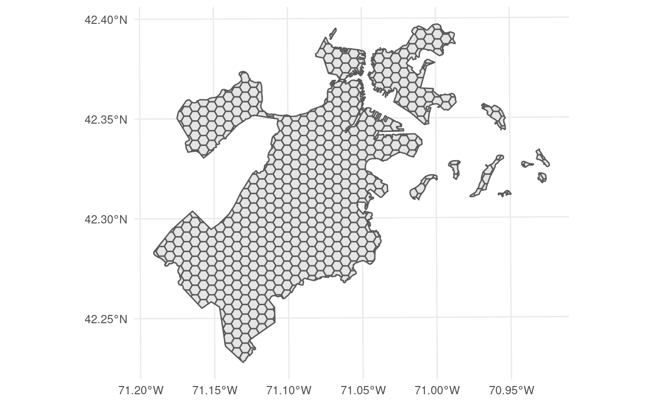
This version of spatialsample includes a new data set, made up of 682 hexagons containing data about tree canopy cover change in Boston, Massachusetts:

library(spatialsample)
library(ggplot2)

ggplot(boston_canopy) + 
  geom_sf()

A map showing the spatial arrangement of hexagons making up the boston_canopy data set.

This data is stored as an sf object, and as such contains information about the proper coordinate reference system and units of measurement associated with the data.

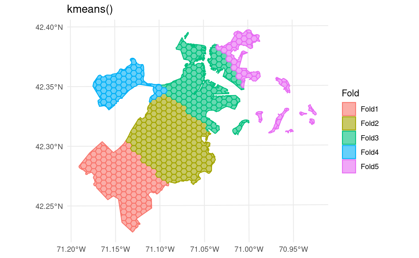
This brings us to the first new feature in this release of spatialsample: spatial_clustering_cv() now supports sf objects, and will calculate distances in a way that respects coordinate reference systems (including using the s2 geometry library for geographic coordinate reference systems):

set.seed(123)
kmeans_clustering <- spatial_clustering_cv(boston_canopy, v = 5)
kmeans_clustering
#> #  5-fold spatial cross-validation 
#> # A tibble: 5 × 2
#>   splits            id   
#>   <list>            <chr>
#> 1 <split [524/158]> Fold1
#> 2 <split [493/189]> Fold2
#> 3 <split [517/165]> Fold3
#> 4 <split [605/77]>  Fold4
#> 5 <split [589/93]>  Fold5

This release also provides autoplot() methods to visualize resamples via ggplot2, making it easy to see how exactly your data is being divided. Just call autoplot() on the outputs from any spatial clustering function:

autoplot(kmeans_clustering) + labs(title = "kmeans()")

A map showing the boston_canopy data set broken into five folds through spatial_clustering_cv. The five folds are visibly different sizes, and are grouped by spatial proximity.

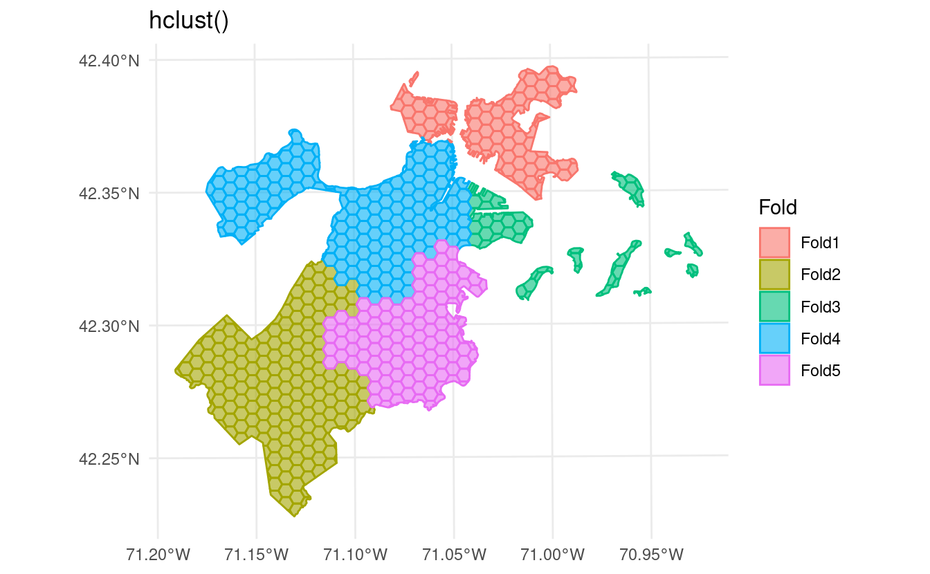
In addition to supporting more types of data, spatial_clustering_cv() has also been extended to support more types of clustering. Set the cluster_function argument to use "hclust" for hierarchical clustering via hclust() instead of the default kmeans()-based clusters:

set.seed(123)
spatial_clustering_cv(
  boston_canopy, 
  v = 5, 
  cluster_function = "hclust"
) |> 
  autoplot() + 
  labs(title = "hclust()")

A map showing the boston_canopy data set broken into five folds through spatial_clustering_cv, using the hclust clustering method. The five folds are still visibly different sizes, and are grouped by spatial proximity, but the clusters are notably different from those produced by the default kmeans method.

This argument can also accept functions, letting you plug in clustering methodologies from other packages or that you’ve written yourself:

set.seed(123)

custom_clusters <- function(dists, v, ...) {
  rep(letters[1:v], length.out = nrow(boston_canopy))
}

spatial_clustering_cv(
  boston_canopy, 
  v = 5, 
  cluster_function = custom_clusters
) |> 
  autoplot() + 
  labs(title = "custom_clusters()")

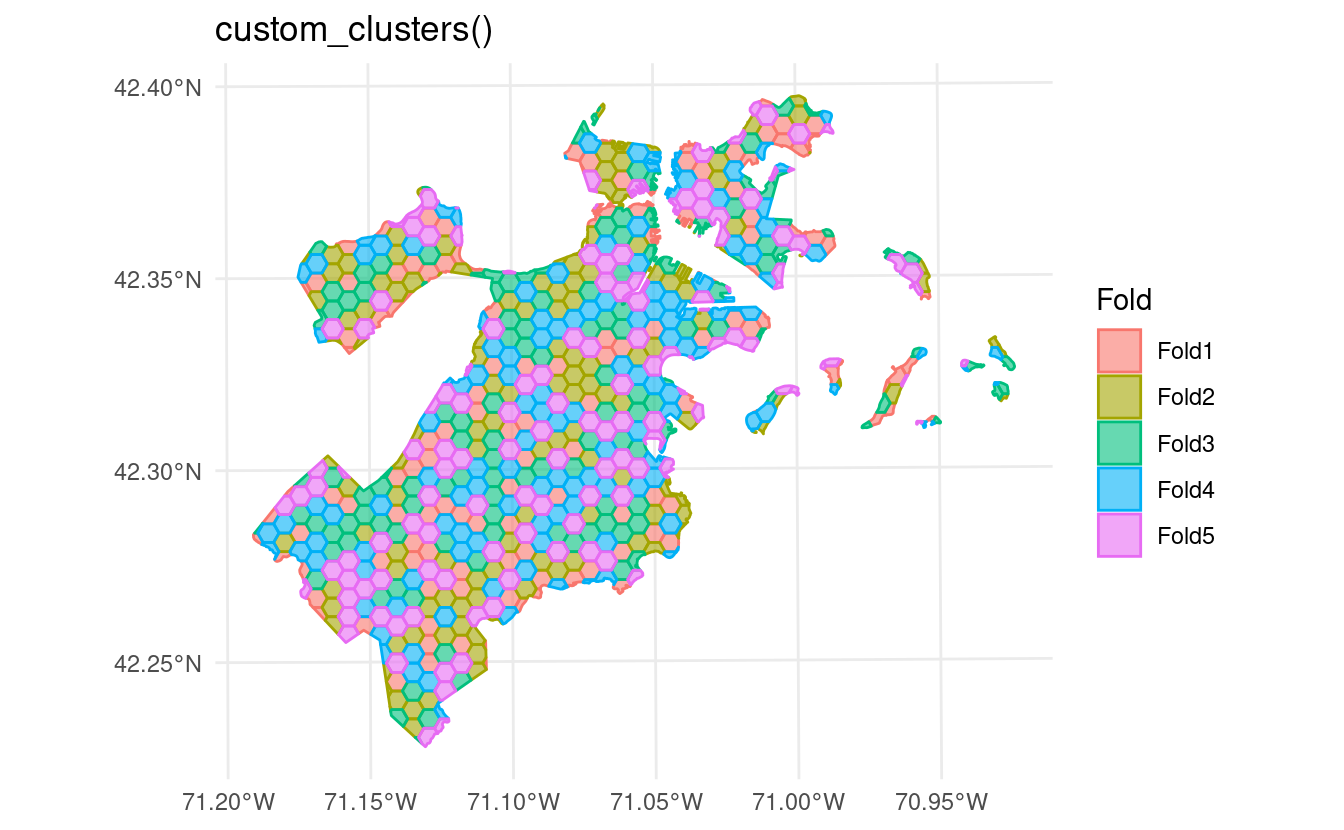
A map showing the outputs of spatial_clustering_cv when using a custom clustering function. The custom clustering function assigned folds systematically, moving sequentially through rows in the data frame, and as such the output does not look very clustered. However, the functions in spatialsample performed exactly the same with the custom clustering function as they did with the built-in options.

In addition to the clustering extensions, this version of spatialsample introduces new functions for other popular spatial resampling methods. For instance, spatial_block_cv() helps you perform block cross-validation, splitting your data into folds based on a grid of regular polygons. You can assign these polygons to folds at random:

set.seed(123)
spatial_block_cv(boston_canopy, v = 5) |> 
  autoplot()

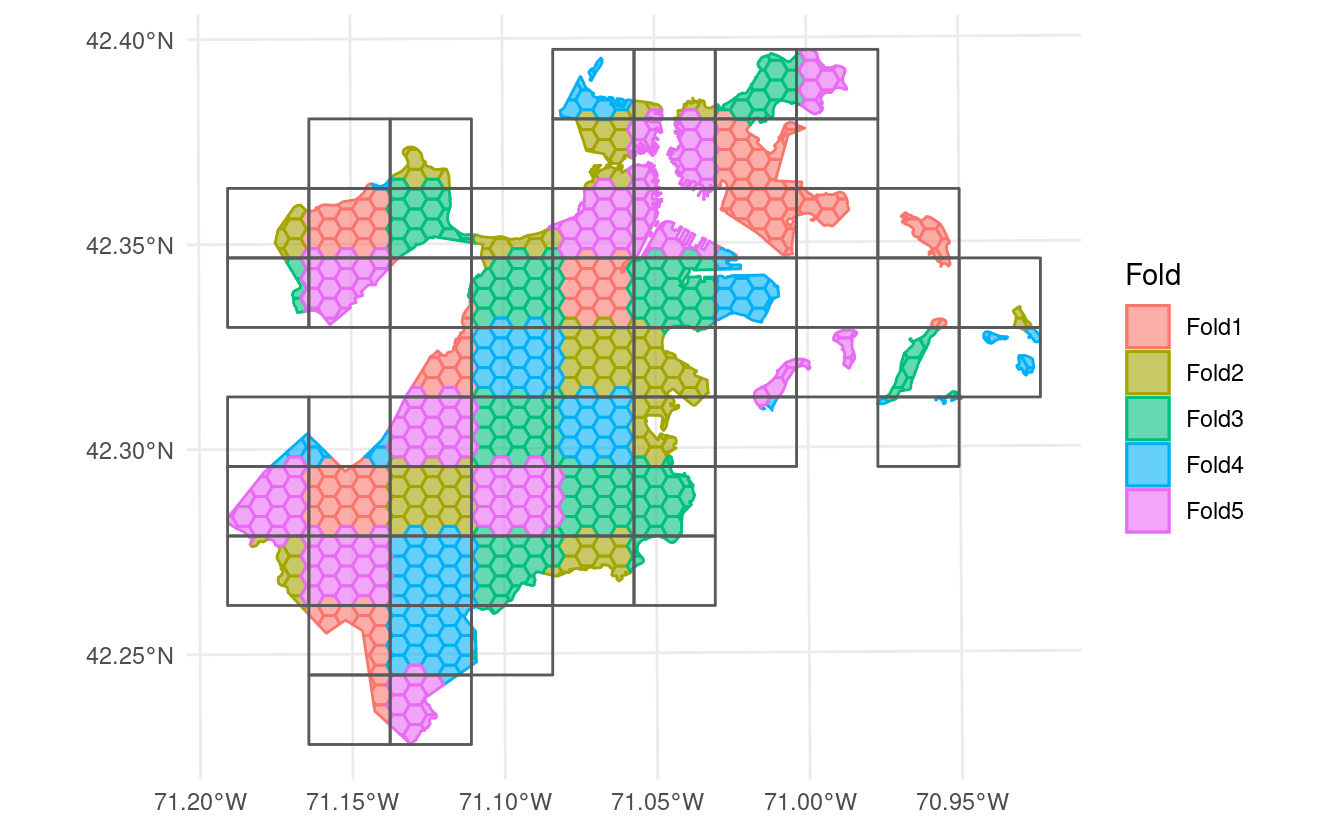
A map showing the outputs of block cross-validation performed using spatial_block_cv. A regular grid of squares has been drawn over the boston_canopy data set, and all data falling into a single block is assigned to the same fold. Blocks are assigned to folds at random, resulting in a patchy distribution of folds across the data set.

Or systematically, either by assigning folds in order from the bottom-left and proceeding from left to right along each row by setting method = "continuous":

spatial_block_cv(boston_canopy, v = 5, method = "continuous") |> 
  autoplot()

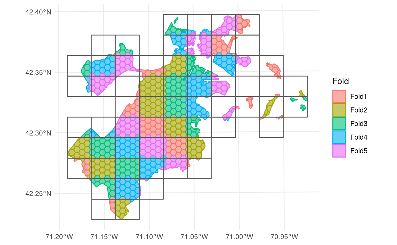
A map showing the outputs of block cross-validation performed using spatial_block_cv with continuous systematic assignment. Rather than the patchy random assignment before, blocks are now assigned from left to right for each row of the regular grid, resulting in the same folds always being adjacent to one another.

Or by “snaking” back and forth up the grid by setting method = "snake":

spatial_block_cv(boston_canopy, v = 5, method = "snake") |> 
  autoplot()

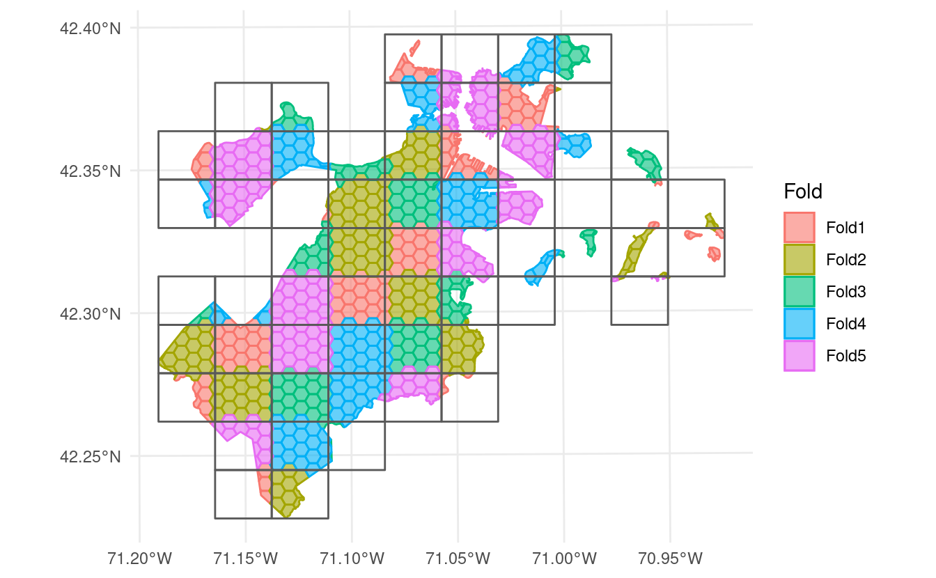
A map showing the outputs of block cross-validation performed using spatial_block_cv with snaking systematic assignment. Blocks are now assigned alternatively from left to right and right to left, resulting in a similar alignment of folds to the continuous method.

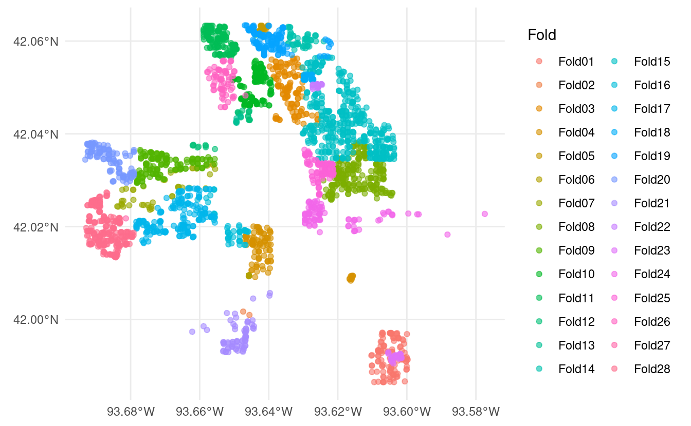
This release of spatialsample also adds support for leave-location-out cross-validation through the new function spatial_leave_location_out_cv(). You can use this to create resamples when you already have a good idea of what data might be spatially correlated together – for instance, we can use it to split the Ames housing data from modeldata by neighborhood:

data(ames, package = "modeldata")

ames_sf <- sf::st_as_sf(ames, coords = c("Longitude", "Latitude"), crs = 4326)

set.seed(123)
spatial_leave_location_out_cv(ames_sf, Neighborhood) |> 
  autoplot()

A map showing the outputs of leave-location-out cross-validation performed using spatial_leave_location_out_cv on the Ames housing data. Folds are assigned based on what neighborhood each house falls into. Some neighborhoods are entirely contained within another neighborhood, and neighborhoods contain very different numbers of houses.

Buffering

The last major feature in this release is the introduction of spatial buffering. Spatial buffering enforces a certain minimum distance between your analysis and assessment sets, making sure that you’re spatially extrapolating when making predictions with a model.

While all spatial resampling functions in spatialsample can use spatial buffers, particularly interesting is the new spatial_buffer_vfold_cv() function. This function makes it easy to add spatial buffers around a standard V-fold cross-validation procedure. When we plot the object returned by this function, it just looks like a standard V-fold cross-validation setup:

set.seed(123)
blocks <- spatial_buffer_vfold_cv(
  boston_canopy, 
  v = 15,
  buffer = 100,
  radius = NULL
)

autoplot(blocks)

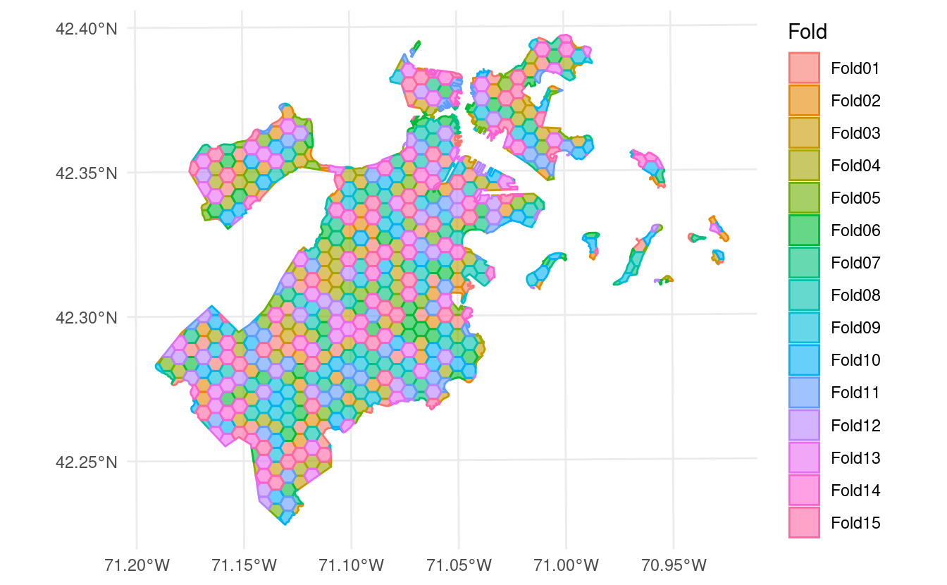
A map showing the outputs of spatially buffered cross-validation performed using spatial_buffer_vfold_cv, once again using the boston_canopy data set. When visualizing all folds at once, there does not seem to be any spatial structure to the resamples; folds are distributed randomly throughout the data set, and folds abut one another without any spatial separation.

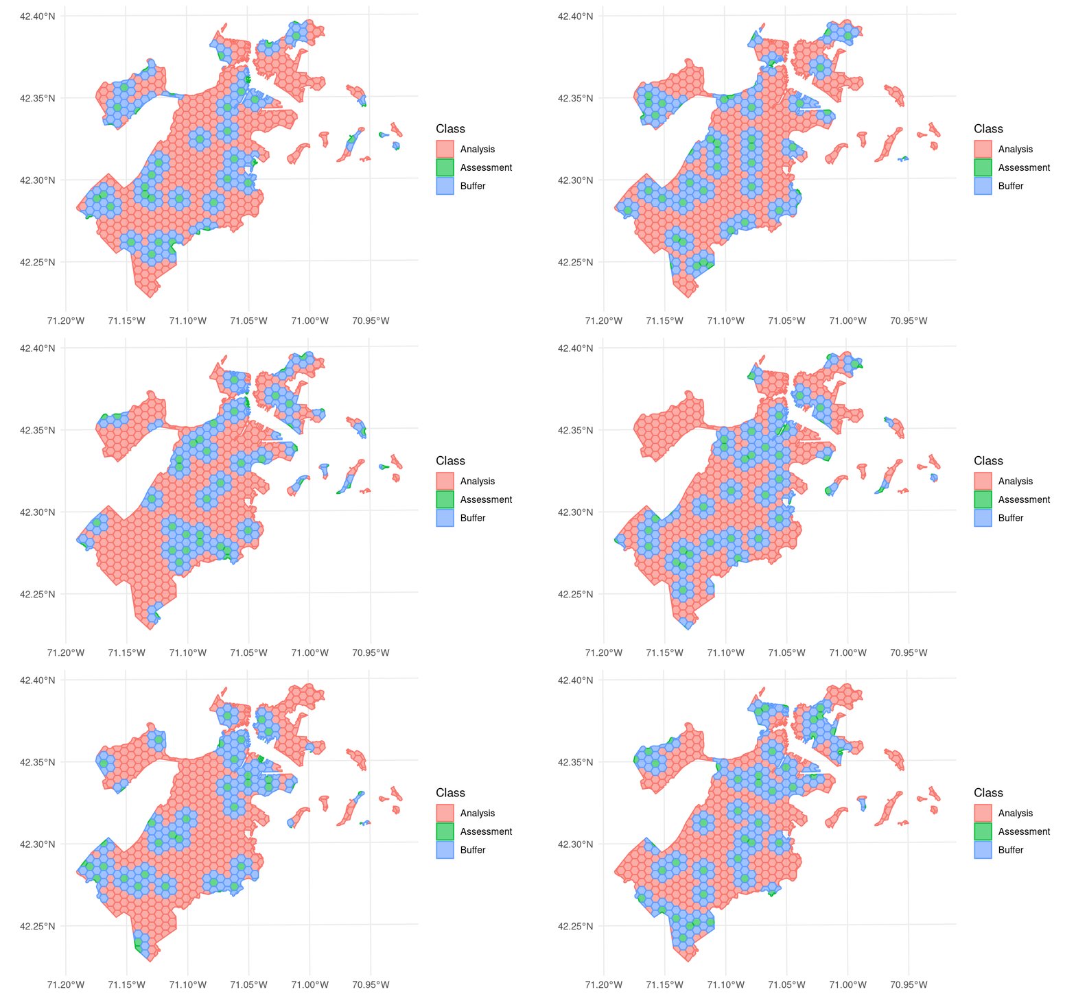
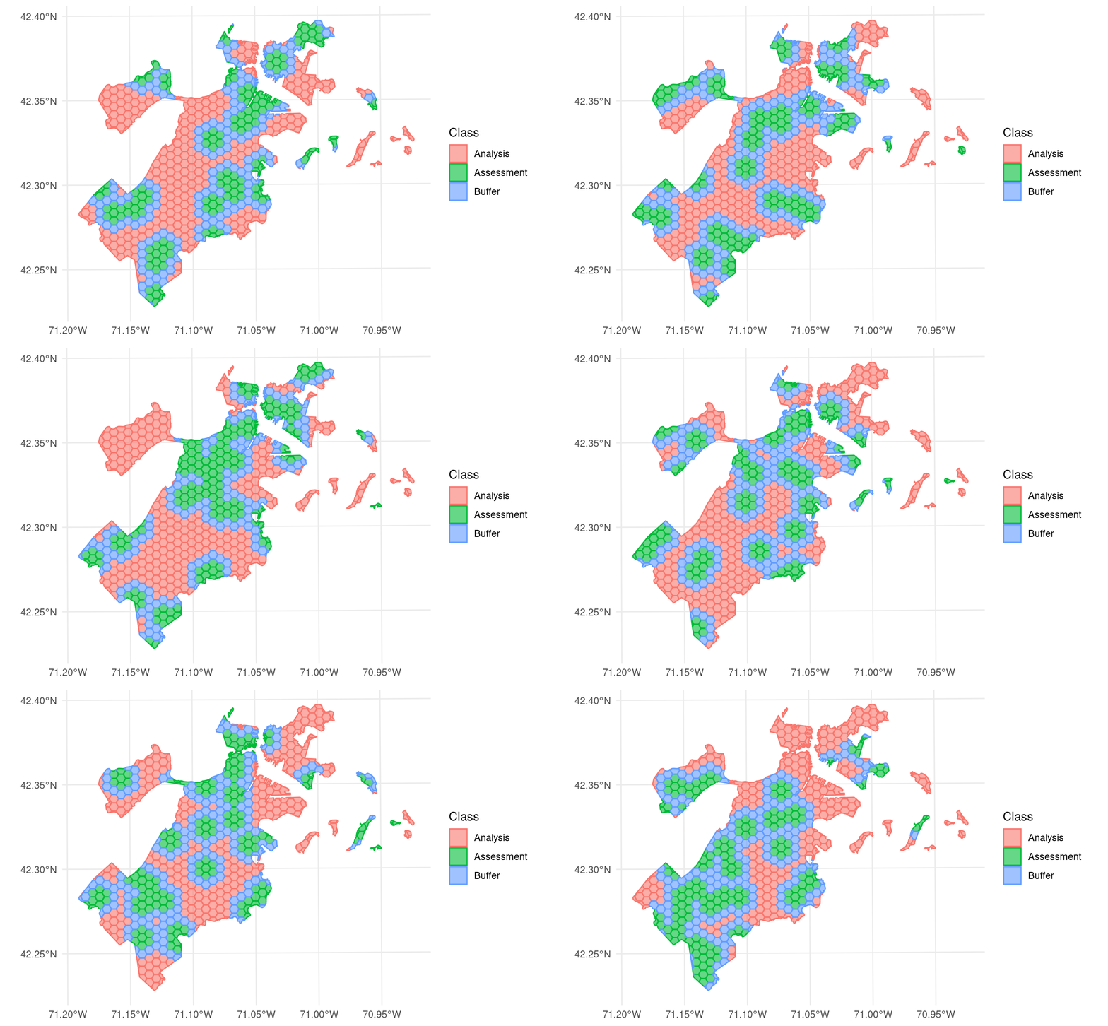
However, if we use autoplot() to visualize the splits themselves, we can see that we’ve created an exclusion buffer around each of our assessment sets. Data inside this buffer is assigned to neither the assessment or analysis set, so you can be sure your data is spatially separated:

blocks$splits |> 
  purrr::walk(function(x) print(autoplot(x)))

An animation showing maps of each individual fold produced using spatial_buffer_vfold_cv. Now it is evident that any data adjacent to the assessment data has been added to a 'buffer' zone, and is part of neither the analysis or the assessment set.

In addition to exclusion buffers, spatialsample now lets you add inclusion radii to any spatial resampling. This will add any points within a certain distance of the original assessment set to the assessment set, letting you create clumped “discs” of data to assess your models against:

set.seed(123)
blocks <- spatial_buffer_vfold_cv(
  boston_canopy, 
  v = 20,
  buffer = 100,
  radius = 100
)

blocks$splits |> 
  purrr::walk(function(x) print(autoplot(x)))

Another animation showing maps of each individual fold produced using spatial_buffer_vfold_cv. When using the argument radius, points adjacent to the assessment set are themselves added to the assessment set. The buffer is then applied to each data point in the enlarged assessment set.

…and more!

This is just scratching the surface of the new features and improvements in this release of spatialsample. You can see a full list of changes in the the release notes.

Acknowledgments

We’d like to thank everyone that has contributed since the last release: @jennybc, @juliasilge, @mikemahoney218, @MxNl, @nipnipj, and @PathosEthosLogos.