
We’re super excited announce the release of infer 1.0.0! infer is a package for statistical inference that implements an expressive statistical grammar that adheres to the tidyverse design framework. Rather than providing methods for specific statistical tests, this package consolidates the principles that are shared among common hypothesis tests and confidence intervals into a set of four main verbs (functions), supplemented with many utilities to visualize and extract value from their outputs. The expressive grammar is specifically designed to allow users to make explicit connections between the computational procedures and the theory of statistical inference, making this package particularly well suited for teaching this topic.
You can install it from CRAN with:
install.packages("infer")This release includes a number of major changes and new features. Namely:
- Support for multiple regression
- Alignment of theory-based methods with their simulation-based counterparts
- Improvements to behavorial consistency of
calculate()
The infer package has been on CRAN since 2017. However, we haven’t written about the package on the tidyverse blog before. Thus, I’ll start out by demonstrating the basics of the package. After, I’ll highlight some of the more neat features introduced in this version of the package. You can find a full list of changes in version 1.0.0 of the package in the release notes.
We also load the tidyverse collection of packages to help with data exploration and manipulation.
library(tidyverse)
#> ── Attaching packages ─────────────────────────────────────── tidyverse 1.3.1 ──
#> ✔ ggplot2 3.3.5     ✔ purrr   0.3.4
#> ✔ tibble  3.1.3     ✔ dplyr   1.0.7
#> ✔ tidyr   1.1.3     ✔ stringr 1.4.0
#> ✔ readr   2.0.1     ✔ forcats 0.5.1
#> ── Conflicts ────────────────────────────────────────── tidyverse_conflicts() ──
#> ✖ dplyr::filter() masks stats::filter()
#> ✖ dplyr::lag()    masks stats::lag()
Getting to know infer
Regardless of the hypothesis test in question, an analyst asks the same kind of question when conducting statistical inference: is the effect/difference in the observed data real, or due to random chance? To answer this question, the analyst begins by assuming that the effect in the observed data was simply due to random chance, and calls this assumption the null hypothesis. (In reality, they might not believe in the null hypothesis at all—the null hypothesis is in opposition to the alternate hypothesis, which supposes that the effect present in the observed data is actually due to the fact that “something is going on.") The analyst then calculates a test statistic from the data that describes the observed effect. They can use this test statistic to calculate a p-value via juxtaposition with a null distribution, giving the probability that the observed data could come about if the null hypothesis were true. If this probability is below some pre-defined significance level $\alpha$, then the analyst can reject the null hypothesis.
The workflow of this package is designed around this idea. Starting out with some dataset,
specify()allows the analyst to specify the variable, or relationship between variables, that they are interested in.hypothesize()allows the analyst to declare the null hypothesis.generate()allows the analyst to generate data reflecting the null hypothesis or using the bootstrap.calculate()allows the analyst to calculate summary statistics, either from- the observed data, to form the observed statistic.
- data
generate()d to reflect the null hypothesis, to form a randomization-based null distribution of statistics. - data
generate()d to form a bootstrap distribution of statistics
As such, the ultimate output of an infer pipeline using these four functions is generally an observed statistic or null distribution of test statistics. These four functions are thus supplemented with several utilities to visualize and extract value from their outputs.
visualize()plots the null distribution of test statistics.shade_p_value()situates the observed statistic in the null distribution, shading the region as or more extreme.
get_p_value()calculates a p-value via the juxtaposition of the test statistic and null distribution.
The workflow outlined above can also be used for constructing confidence intervals via bootstrapping with the omission of the
hypothesize() step in the pipeline. The resulting bootstrap distribution can then be visualized with
visualize(), the confidence interval region can be situated in the bootstrap distribution with
shade_confidence_interval(), and the bounds of the confidence interval can be calculated with
get_confidence_interval().
To demonstrate, we’ll walk through a typical infer pipeline step-by-step. Throughout this post, we make use of gss, a dataset supplied by infer containing a sample of 500 observations of 11 variables from the General Social Survey.
# take a look at its structure
glimpse(gss)
#> Rows: 500
#> Columns: 11
#> $ year    <dbl> 2014, 1994, 1998, 1996, 1994, 1996, 1990, 2016, 2000, 1998, 20…
#> $ age     <dbl> 36, 34, 24, 42, 31, 32, 48, 36, 30, 33, 21, 30, 38, 49, 25, 56…
#> $ sex     <fct> male, female, male, male, male, female, female, female, female…
#> $ college <fct> degree, no degree, degree, no degree, degree, no degree, no de…
#> $ partyid <fct> ind, rep, ind, ind, rep, rep, dem, ind, rep, dem, dem, ind, de…
#> $ hompop  <dbl> 3, 4, 1, 4, 2, 4, 2, 1, 5, 2, 4, 3, 4, 4, 2, 2, 3, 2, 1, 2, 5,…
#> $ hours   <dbl> 50, 31, 40, 40, 40, 53, 32, 20, 40, 40, 23, 52, 38, 72, 48, 40…
#> $ income  <ord> $25000 or more, $20000 - 24999, $25000 or more, $25000 or more…
#> $ class   <fct> middle class, working class, working class, working class, mid…
#> $ finrela <fct> below average, below average, below average, above average, ab…
#> $ weight  <dbl> 0.8960034, 1.0825000, 0.5501000, 1.0864000, 1.0825000, 1.08640…
Each row is an individual survey response, containing some basic demographic information on the respondent as well as some additional variables. See
?gss for more information on the variables included and their source.
specify(): Specifying response (and explanatory) variables
The
specify() function can be used to specify which of the variables in the dataset you’re interested in. If you’re only interested in, say, the age of the respondents, you might write:
gss %>%
  specify(response = age)
#> Response: age (numeric)
#> # A tibble: 500 × 1
#>      age
#>    <dbl>
#>  1    36
#>  2    34
#>  3    24
#>  4    42
#>  5    31
#>  6    32
#>  7    48
#>  8    36
#>  9    30
#> 10    33
#> # … with 490 more rows
On the front end, the output of
specify() just looks like it selects off the columns in the dataframe that you’ve specified. Checking the class of this object, though:
We can see that the infer class has been appended on top of the dataframe classes–this new class stores some extra metadata.
If you’re interested in two variables–age and partyid, for example–you can
specify() their relationship in one of two (equivalent) ways:
# as a formula
gss %>%
  specify(age ~ partyid)
#> Response: age (numeric)
#> Explanatory: partyid (factor)
#> # A tibble: 500 × 2
#>      age partyid
#>    <dbl> <fct>
#>  1    36 ind
#>  2    34 rep
#>  3    24 ind
#>  4    42 ind
#>  5    31 rep
#>  6    32 rep
#>  7    48 dem
#>  8    36 ind
#>  9    30 rep
#> 10    33 dem
#> # … with 490 more rows

# with the named arguments
gss %>%
  specify(response = age, explanatory = partyid)
#> Response: age (numeric)
#> Explanatory: partyid (factor)
#> # A tibble: 500 × 2
#>      age partyid
#>    <dbl> <fct>
#>  1    36 ind
#>  2    34 rep
#>  3    24 ind
#>  4    42 ind
#>  5    31 rep
#>  6    32 rep
#>  7    48 dem
#>  8    36 ind
#>  9    30 rep
#> 10    33 dem
#> # … with 490 more rows
hypothesize(): Declaring the null hypothesis
The next step in an infer pipeline is often to declare a null hypothesis using
hypothesize(). The first step is to supply one of “independence” or “point” to the null argument. If your null hypothesis assumes independence between two variables, then this is all you need to supply to
hypothesize():
gss %>%
  specify(college ~ partyid, success = "degree") %>%
  hypothesize(null = "independence")
#> Response: college (factor)
#> Explanatory: partyid (factor)
#> Null Hypothesis: independence
#> # A tibble: 500 × 2
#>    college   partyid
#>    <fct>     <fct>
#>  1 degree    ind
#>  2 no degree rep
#>  3 degree    ind
#>  4 no degree ind
#>  5 degree    rep
#>  6 no degree rep
#>  7 no degree dem
#>  8 degree    ind
#>  9 degree    rep
#> 10 no degree dem
#> # … with 490 more rows
If you’re doing inference on a point estimate, you will also need to provide one of p (the true proportion of successes, between 0 and 1), mu (the true mean), med (the true median), or sigma (the true standard deviation). For instance, if the null hypothesis is that the mean number of hours worked per week in our population is 40, we would write:
gss %>%
  specify(response = hours) %>%
  hypothesize(null = "point", mu = 40)
#> Response: hours (numeric)
#> Null Hypothesis: point
#> # A tibble: 500 × 1
#>    hours
#>    <dbl>
#>  1    50
#>  2    31
#>  3    40
#>  4    40
#>  5    40
#>  6    53
#>  7    32
#>  8    20
#>  9    40
#> 10    40
#> # … with 490 more rows
Again, on the front end, the dataframe outputted from
hypothesize() looks almost exactly the same as it did when it came out of
specify(), but infer now “knows” your null hypothesis.
generate(): Generating the simulated distribution
Once we’ve asserted our null hypothesis using
hypothesize(), we can construct a null distribution based on this hypothesis. We can do this using one of several methods, supplied in the type argument:
permute: For each replicate, each input value will be randomly reassigned (without replacement) to a new output value in the sample.draw: A value will be sampled from a theoretical distribution with parameters specified inhypothesize()for each replicate. (This option is currently only applicable for testing point estimates.)bootstrap: A bootstrap sample will be drawn for each replicate, where a sample of size equal to the input sample size is drawn (with replacement) from the input sample data. The bootstrap is most commonly used in the context of constructing a confidence interval, omitting infer’shypothesize()step.
Continuing on with our example above, about the average number of hours worked a week, we might write:
gss %>%
  specify(response = hours) %>%
  hypothesize(null = "point", mu = 40) %>%
  generate(reps = 1000, type = "bootstrap")
#> Response: hours (numeric)
#> Null Hypothesis: point
#> # A tibble: 500,000 × 2
#> # Groups:   replicate [1,000]
#>    replicate hours
#>        <int> <dbl>
#>  1         1 46.6
#>  2         1 37.6
#>  3         1 58.6
#>  4         1 38.6
#>  5         1 28.6
#>  6         1 35.6
#>  7         1 43.6
#>  8         1  6.62
#>  9         1 48.6
#> 10         1 53.6
#> # … with 499,990 more rows
In the above example, we take 1000 bootstrap samples to form our null distribution.
To generate a null distribution for the independence of two variables, we could randomly reshuffle the pairings of explanatory and response variables to break any existing association. For instance, to generate 1000 replicates that can be used to create a null distribution under the assumption that political party affiliation is not affected by age:
gss %>%
  specify(partyid ~ age) %>%
  hypothesize(null = "independence") %>%
  generate(reps = 1000, type = "permute")
#> Response: partyid (factor)
#> Explanatory: age (numeric)
#> Null Hypothesis: independence
#> # A tibble: 500,000 × 3
#> # Groups:   replicate [1,000]
#>    partyid   age replicate
#>    <fct>   <dbl>     <int>
#>  1 rep        36         1
#>  2 dem        34         1
#>  3 dem        24         1
#>  4 dem        42         1
#>  5 ind        31         1
#>  6 ind        32         1
#>  7 ind        48         1
#>  8 dem        36         1
#>  9 ind        30         1
#> 10 ind        33         1
#> # … with 499,990 more rows
calculate(): Calculating summary statistics
calculate() calculates summary statistics from the output of infer core functions. The function, for one, takes in a stat argument, which is currently one of "mean", "median", "sum", "sd", "prop", "count", "diff in means", "diff in medians", "diff in props", "Chisq", "F", "t", "z", "slope", or "correlation". For example, continuing our example above to calculate the null distribution of mean hours worked per week:
gss %>%
  specify(response = hours) %>%
  hypothesize(null = "point", mu = 40) %>%
  generate(reps = 1000, type = "bootstrap") %>%
  calculate(stat = "mean")
#> Response: hours (numeric)
#> Null Hypothesis: point
#> # A tibble: 1,000 × 2
#>    replicate  stat
#>        <int> <dbl>
#>  1         1  38.6
#>  2         2  40.4
#>  3         3  38.9
#>  4         4  40.0
#>  5         5  39.7
#>  6         6  40.0
#>  7         7  40.9
#>  8         8  40.4
#>  9         9  41.7
#> 10        10  39.8
#> # … with 990 more rows
The output of
calculate() here shows us the sample statistic (in this case, the mean) for each of our 1000 replicates. To calculate the mean from the observed data, just omit the
hypothesize() and
generate() steps.
gss %>%
  specify(response = hours) %>%
  calculate(stat = "mean")
#> Response: hours (numeric)
#> # A tibble: 1 × 1
#>    stat
#>   <dbl>
#> 1  41.4
Other utilities
infer offers several utilities to extract meaning from summary statistics and distributions—the package provides functions to visualize where a statistic is relative to a distribution (with
visualize()), calculate p-values (with
get_p_value()), and calculate confidence intervals (with
get_confidence_interval()).
To illustrate, we’ll go back to the example of determining whether the mean number of hours worked per week is 40 hours.
# find the point estimate
point_estimate <- gss %>%
  specify(response = hours) %>%
  calculate(stat = "mean")

# generate a distribution of means
dist <- gss %>%
  specify(response = hours) %>%
  hypothesize(null = "point", mu = 40) %>%
  generate(reps = 1000, type = "bootstrap") %>%
  calculate(stat = "mean")
Our point estimate 41.382 seems pretty close to 40, but a little bit different. We might wonder if this difference is just due to random chance, or if the mean number of hours worked per week in the population really isn’t 40.
We could initially just visualize the distribution.
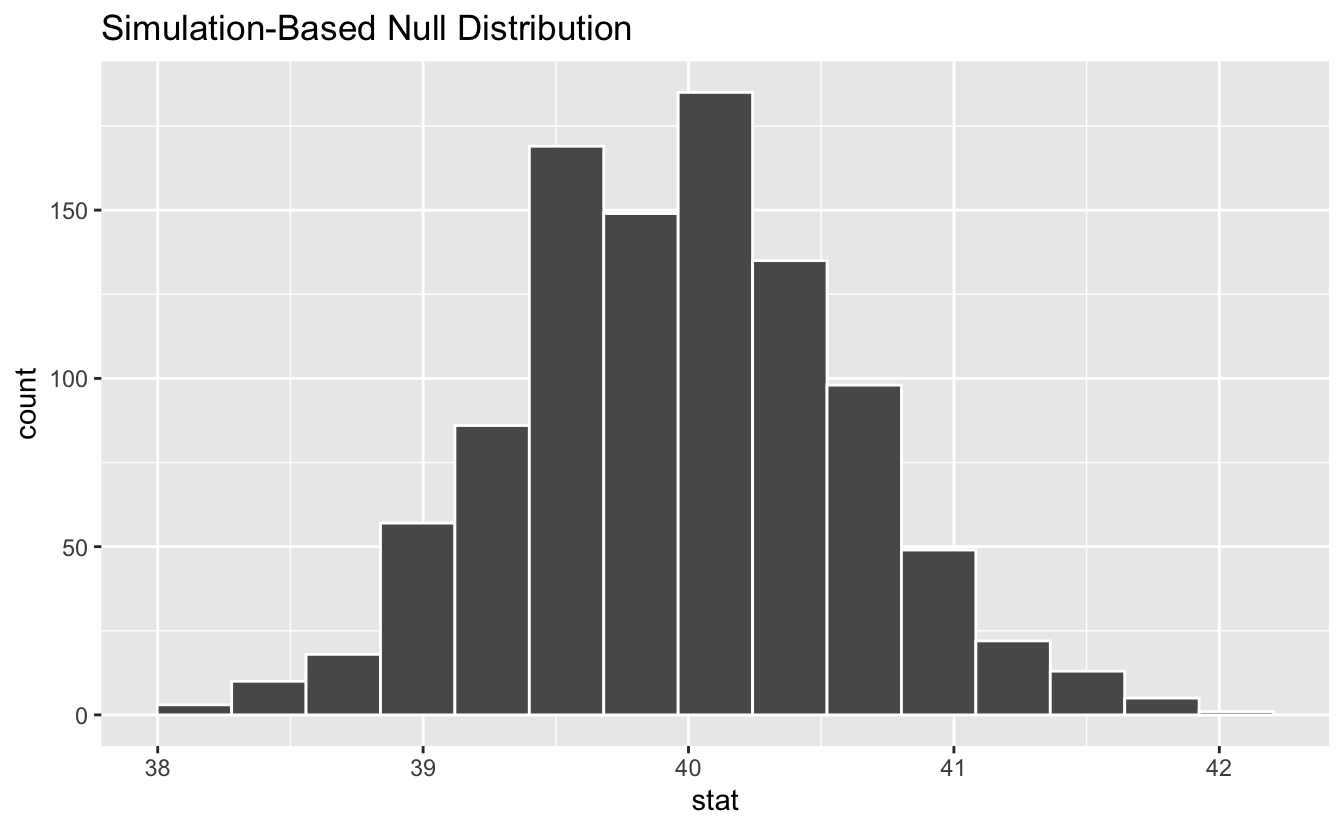
Where does our sample’s observed statistic lie on this distribution? We can use the obs_stat argument to specify this.
dist %>%
visualize() +
shade_p_value(obs_stat = point_estimate, direction = "two-sided")
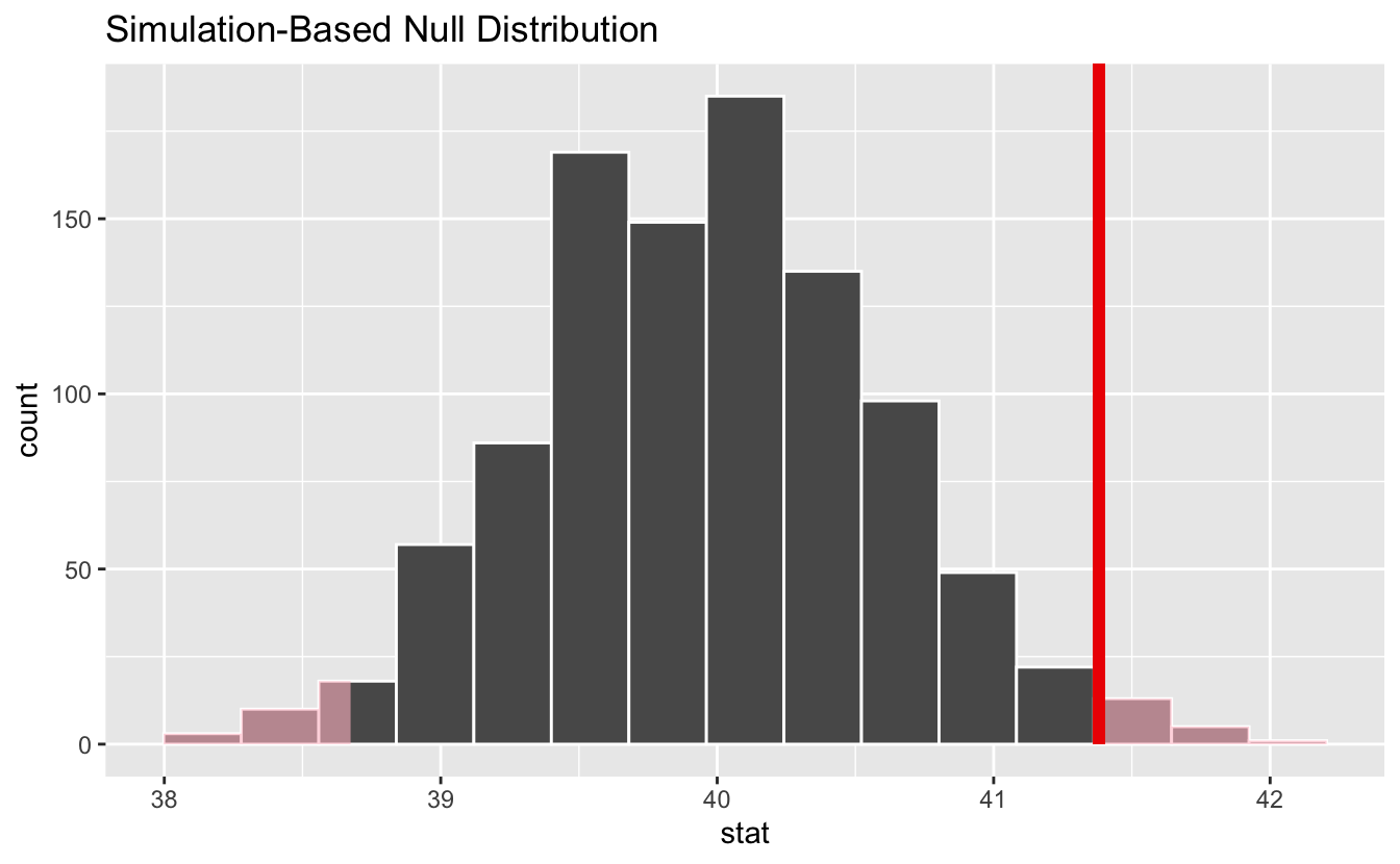
Notice that infer has also shaded the regions of the null distribution that are as (or more) extreme than our observed statistic. The red bar looks like it’s slightly far out on the right tail of the null distribution, so observing a sample mean of 41.382 hours would be somewhat unlikely if the mean was actually 40 hours. How unlikely, though?
p_value <- dist %>%
  get_p_value(obs_stat = point_estimate, direction = "two-sided")

p_value
#> # A tibble: 1 × 1
#>   p_value
#>     <dbl>
#> 1   0.038
It looks like the p-value is 0.038, which is pretty small—if the true mean number of hours worked per week was actually 40, the probability of our sample mean being this far (1.382 hours) from 40 would be 0.038. This may or may not be statistically significantly different, depending on the significance level $\alpha$ you decided on before you ran this analysis. If you had set $\alpha = 0.05$, then this difference would be statistically significant, but if you had set $\alpha = 0.01$, then it would not be.
To get a confidence interval around our estimate, we can write:
dist %>%
  get_confidence_interval(
    point_estimate = point_estimate,
    level = 0.95,
    type = "se"
  )
#> # A tibble: 1 × 2
#>   lower_ci upper_ci
#>      <dbl>    <dbl>
#> 1     40.1     42.6
As you can see, 40 hours per week is not contained in this interval, which aligns with our previous conclusion that this finding is significant at the confidence level $\alpha = 0.05$.
What’s new?
There are a number of improvements and new features in this release that resolve longstanding gaps in the package’s functionality. We’ll highlight three:
- Support for multiple regression
- Alignment of theory-based methods
- Behavioral consistency of
calculate()
Support for multiple regression
The 2016 “Guidelines for Assessment and Instruction in Statistics Education” [1] state that, in introductory statistics courses, “[s]tudents should gain experience with how statistical models, including multivariable models, are used.” In line with this recommendation, we introduce support for randomization-based inference with multiple explanatory variables via a new fit.infer core verb.
If passed an infer object, the method will parse a formula out of the formula or response and explanatory arguments, and pass both it and data to a
stats::glm call.
gss %>%
  specify(hours ~ age + college) %>%
  fit()
#> # A tibble: 3 × 2
#>   term          estimate
#>   <chr>            <dbl>
#> 1 intercept     40.6
#> 2 age            0.00596
#> 3 collegedegree  1.53
Note that the function returns the model coefficients as estimate rather than their associated $t$-statistics as stat.
If passed a
generate()d object, the model will be fitted to each replicate.
gss %>%
  specify(hours ~ age + college) %>%
  hypothesize(null = "independence") %>%
  generate(reps = 100, type = "permute") %>%
  fit()
#> # A tibble: 300 × 3
#> # Groups:   replicate [100]
#>    replicate term          estimate
#>        <int> <chr>            <dbl>
#>  1         1 intercept     41.5
#>  2         1 age            0.0139
#>  3         1 collegedegree -1.88
#>  4         2 intercept     40.6
#>  5         2 age           -0.00221
#>  6         2 collegedegree  2.64
#>  7         3 intercept     40.5
#>  8         3 age            0.0196
#>  9         3 collegedegree  0.251
#> 10         4 intercept     39.3
#> # … with 290 more rows
If type = "permute", a set of unquoted column names in the data to permute (independently of each other) can be passed via the variables argument to generate. It defaults to only the response variable.
gss %>%
  specify(hours ~ age + college) %>%
  hypothesize(null = "independence") %>%
  generate(reps = 100, type = "permute", variables = c(age, college)) %>%
  fit()
#> # A tibble: 300 × 3
#> # Groups:   replicate [100]
#>    replicate term          estimate
#>        <int> <chr>            <dbl>
#>  1         1 intercept      44.4
#>  2         1 age            -0.0774
#>  3         1 collegedegree   0.366
#>  4         2 intercept      40.7
#>  5         2 age             0.0124
#>  6         2 collegedegree   0.613
#>  7         3 intercept      40.0
#>  8         3 age             0.0306
#>  9         3 collegedegree   0.496
#> 10         4 intercept      40.9
#> # … with 290 more rows
This feature allows for more detailed exploration of the effect of disrupting the correlation structure among explanatory variables on outputted model coefficients.
Each of the auxillary functions
get_p_value(),
get_confidence_interval(),
visualize(),
shade_p_value(), and
shade_confidence_interval() have methods to handle
fit() output! See their help-files for example usage.
Alignment of theory-based methods
While infer is primarily a package for randomization-based statistical inference, the package has partially supported theory-based methods in a number of ways over the years. This release introduces a principled, opinionated, and consistent interface for theory-based methods for statistical inference. The new interface is based on a new verb,
assume(), that returns a distribution that, once created, interfaces in the same way that simulation-based distributions do.
To demonstrate, we’ll return to the example of inference on a mean using infer’s gss dataset. Supposed that we believe the true mean number of hours worked by Americans in the past week is 40.
First, calculating the observed $t$-statistic:
obs_stat <- gss %>%
  specify(response = hours) %>%
  hypothesize(null = "point", mu = 40) %>%
  calculate(stat = "t")

obs_stat
#> Response: hours (numeric)
#> Null Hypothesis: point
#> # A tibble: 1 × 1
#>    stat
#>   <dbl>
#> 1  2.09
The code to define the null distribution is very similar to that required to calculate a theorized observed statistic, switching out
calculate() for
assume() and adjusting arguments as needed.
dist <- gss %>%
  specify(response = hours) %>%
  hypothesize(null = "point", mu = 40) %>%
  assume(distribution = "t")

dist
#> A T distribution with 499 degrees of freedom.
This null distribution can now be interfaced with in the same way as a simulation-based null distribution elsewhere in the package. For example, calculating a p-value by juxtaposing the observed statistic and null distribution:
get_p_value(dist, obs_stat, direction = "both")
#> # A tibble: 1 × 1
#> p_value
#> <dbl>
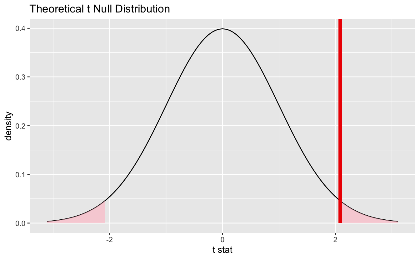
#> 1 0.0376…or juxtaposing the two visually:
visualize(dist) +
  shade_p_value(obs_stat, direction = "both")
Confidence intervals lie on the scale of the observed data rather than the standardized scale of the theoretical distributions. Calculating a mean rather than the standardized $t$-statistic:
obs_mean <- gss %>%
  specify(response = hours) %>%
  calculate(stat = "mean")

obs_mean
#> Response: hours (numeric)
#> # A tibble: 1 × 1
#>    stat
#>   <dbl>
#> 1  41.4
The distribution here just defines the spread for the standard error calculation.
ci <-
get_confidence_interval(
dist,
level = 0.95,
point_estimate = obs_mean
)
ci
#> # A tibble: 1 × 2
#> lower_ci upper_ci
#> <dbl> <dbl>
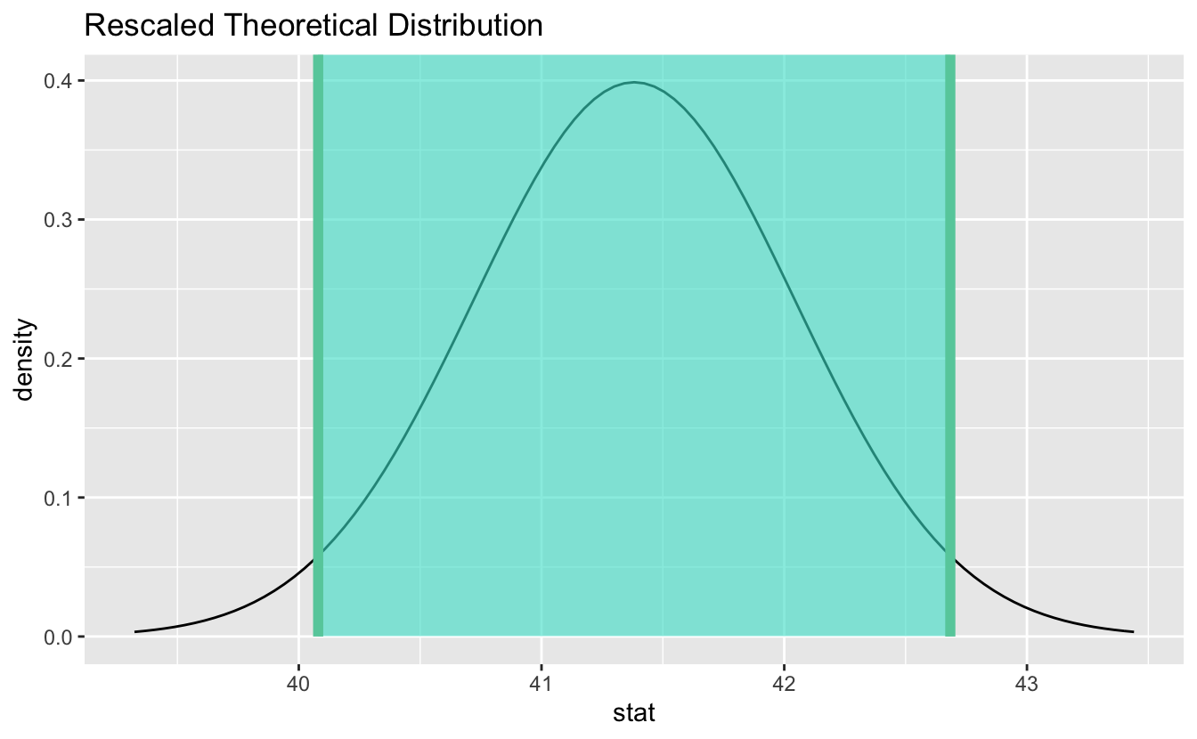
#> 1 40.1 42.7Visualizing the confidence interval results in the theoretical distribution being recentered and rescaled to align with the scale of the observed data:
visualize(dist) +
  shade_confidence_interval(ci)
Previous methods for interfacing with theoretical distributions are superseded—they will continue to be supported, though documentation will forefront the
assume() interface.
Behavioral consistency
Another major change to the package in this release is a set of standards for behavorial consistency of
calculate(). Namely, the package will now
supply a consistent error when the supplied
statargument isn’t well-defined for the variablesspecify()dgss %>% specify(response = hours) %>% calculate(stat = "diff in means") #> Error: A difference in means is not well-defined for a numeric response variable (hours) and no explanatory variable.or
gss %>%
    specify(college ~ partyid, success = "degree") %>%
    calculate(stat = "diff in props")
  #> Dropping unused factor levels DK from the supplied explanatory variable 'partyid'.
  #> Error: A difference in proportions is not well-defined for a dichotomous categorical response variable (college) and a multinomial categorical explanatory variable (partyid).
supply a consistent message when the user supplies unneeded information via
hypothesize()tocalculate()an observed statistic# supply mu = 40 when it's not needed gss %>% specify(response = hours) %>% hypothesize(null = "point", mu = 40) %>% calculate(stat = "mean") #> Message: The point null hypothesis `mu = 40` does not inform calculation of the observed statistic (a mean) and will be ignored. #> Response: hours (numeric) #> Null Hypothesis: point #> # A tibble: 1 × 1 #> stat #> <dbl> #> 1 41.4
and
supply a consistent warning and assume a reasonable null value when the user does not supply sufficient information to calculate an observed statistic
# don't hypothesize `p` when it's needed
  gss %>%
      specify(response = sex, success = "female") %>%
      calculate(stat = "z")
  #> Warning: A z statistic requires a null hypothesis to calculate the observed statistic.
  #> Output assumes the following null value: `p = .5`.
  #> Response: sex (factor)
  #> Null Hypothesis: point
  #> # A tibble: 1 × 1
  #>    stat
  #>   <dbl>
  #> 1 -1.16
or
# don't hypothesize `p` when it's needed
  gss %>%
    specify(response = partyid) %>%
    calculate(stat = "Chisq")
  #> Dropping unused factor levels DK from the supplied response variable 'partyid'.
  #> Warning: A chi-square statistic requires a null hypothesis to calculate the observed statistic.
  #> Output assumes the following null values: `p = c(dem = 0.2, ind = 0.2, rep = 0.2, other = 0.2, DK = 0.2)`.
  #> Response: partyid (factor)
  #> Null Hypothesis: point
  #> # A tibble: 1 × 1
  #>    stat
  #>   <dbl>
  #> 1  334.
We don’t anticipate that any of these changes are “breaking” in the sense that code that previously worked will continue to, though it may now message or warn in a way that it did not used to or error with a different (and hopefully more informative) message.
Acknowledgements
This release was made possible with financial support from RStudio and the Reed College Mathematics Department. Thanks to @aarora79, @acpguedes, @AlbertRapp, @alexpghayes, @aloy, @AmeliaMN, @andrewpbray, @apreshill, @atheobold, @beanumber, @bigdataman2015, @bragks, @brendanhcullen, @CarlssonLeo, @ChalkboardSonata, @chriscardillo, @clauswilke, @congdanh8391, @corinne-riddell, @cristianvaldez, @daranzolin, @davidbaniadam, @davidhodge931, @doug-friedman, @dshelldhillon, @dsolito, @echasnovski, @EllaKaye, @enricochavez, @gdbassett, @ghost, @GitHunter0, @hardin47, @hfrick, @higgi13425, @instantkaffee, @ismayc, @jbourak, @jcvall, @jimrothstein, @kennethban, @m-berkes, @mikelove, @mine-cetinkaya-rundel, @Minhasshazu, @msberends, @mt-edwards, @muschellij2, @nfultz, @nicholasjhorton, @PirateGrunt, @PsychlytxTD, @richierocks, @romainfrancois, @rpruim, @rudeboybert, @rundel, @sastoudt, @sbibauw, @sckott, @THargreaves, @topepo, @torockel, @ttimbers, @vikram-rawat, @vladimirvrabely, and @xiaochi-liu for their contributions to the package.
[1]: GAISE College Report ASA Revision Committee, “Guidelines for Assessment and Instruction in Statistics Education College Report 2016,” http://www.amstat.org/education/gaise.