
We are happy to announce the release of the rules package on CRAN. rules is another “parsnip-adjacent” package that enables a specific class of models within the tidymodels infrastructure. rules currently contains three models:
C5_rules(): classification rule sets based on the C5.0 model.cubist_rules(): regression rules using Cubist.rule_fit(): classification or regression rules using the RuleFit model.
If you aren’t familiar with rule-based models, there is a companion blog post that summarizes how they work.
Install rules from CRAN like so:
install.packages("rules")
Then attach it for use via:
library(rules)
Here’s an example of creating Cubist regression rules via the parsnip package:
library(tidymodels)
#> ── Attaching packages ──────────────────────────────────── tidymodels 0.1.0 ──
#> ✓ broom     0.5.6      ✓ recipes   0.1.12
#> ✓ dials     0.0.6      ✓ rsample   0.0.6
#> ✓ dplyr     0.8.5      ✓ tibble    3.0.1
#> ✓ ggplot2   3.3.0      ✓ tune      0.1.0
#> ✓ infer     0.5.1      ✓ workflows 0.1.1
#> ✓ parsnip   0.1.1      ✓ yardstick 0.0.6
#> ✓ purrr     0.3.4
#> ── Conflicts ─────────────────────────────────────── tidymodels_conflicts() ──
#> x purrr::accumulate() masks foreach::accumulate()
#> x purrr::discard()    masks scales::discard()
#> x dplyr::filter()     masks stats::filter()
#> x dplyr::lag()        masks stats::lag()
#> x ggplot2::margin()   masks dials::margin()
#> x recipes::step()     masks stats::step()
#> x purrr::when()       masks foreach::when()
library(rules)

data(car_prices, package = "modeldata")

set.seed(9932)
car_split <- initial_split(car_prices)
car_tr <- training(car_split)
car_te <-  testing(car_split)

# A single rule set:
cubist_mod <-
  cubist_rules(neighbors = 7) %>%
  set_engine("Cubist")

cubist_fit <-
  cubist_mod %>%
  fit(log10(Price) ~ ., data = car_tr)

summary(cubist_fit$fit)
#>
#> Call:
#> cubist.default(x = x, y = y, committees = 1)
#>
#>
#> Cubist [Release 2.07 GPL Edition]  Wed May 20 21:39:22 2020
#> ---------------------------------
#>
#>     Target attribute `outcome'
#>
#> Read 603 cases (18 attributes) from undefined.data
#>
#> Model:
#>
#>   Rule 1: [210 cases, mean 4.116360, range 3.94295 to 4.2505, est err 0.030756]
#>
#>     if
#> 	Cylinder <= 4
#> 	Saab <= 0
#>     then
#> 	outcome = 4.115185 + 0.12 Saab - 3.5e-06 Mileage + 0.017 Cylinder
#> 	          - 0.087 hatchback - 0.029 Chevy + 0.046 wagon + 0.028 Leather
#> 	          + 0.041 Cadillac - 0.024 sedan + 0.027 convertible
#> 	          + 0.006 Doors + 0.012 Buick
#>
#>   Rule 2: [8 cases, mean 4.207121, range 4.13308 to 4.26696, est err 0.006589]
#>
#>     if
#> 	Cylinder > 4
#> 	Saturn > 0
#>     then
#> 	outcome = 3.88624 + 0.057 Cylinder + 0.2 Saab + 0.141 Cadillac
#> 	          - 3.8e-06 Mileage - 0.054 sedan + 0.094 convertible
#> 	          - 0.085 hatchback + 0.019 Doors + 0.04 Buick + 0.014 Cruise
#> 	          + 0.01 Leather + 0.007 Sound + 0.007 Saturn
#>
#>   Rule 3: [33 cases, mean 4.229076, range 4.16741 to 4.29184, est err 0.012903]
#>
#>     if
#> 	Cylinder > 4
#> 	Cruise <= 0
#>     then
#> 	outcome = 4.265627 - 3.7e-06 Mileage + 0.039 Chevy
#>
#>   Rule 4: [94 cases, mean 4.272727, range 4.18913 to 4.4427, est err 0.034717]
#>
#>     if
#> 	Mileage > 3946
#> 	Cylinder > 4
#> 	Doors > 2
#> 	Cruise > 0
#> 	Buick <= 0
#> 	Cadillac <= 0
#> 	Saturn <= 0
#>     then
#> 	outcome = 4.037203 + 0.051 Cylinder - 4.3e-06 Mileage + 0.061 Saab
#> 	          + 0.044 Cadillac - 0.016 sedan + 0.029 convertible
#> 	          - 0.026 hatchback + 0.006 Doors - 0.009 Chevy + 0.012 Buick
#> 	          + 0.004 Cruise
#>
#>   Rule 5: [57 cases, mean 4.314541, range 4.17208 to 4.42864, est err 0.049758]
#>
#>     if
#> 	Buick > 0
#>     then
#> 	outcome = 4.389884 - 3e-06 Mileage
#>
#>   Rule 6: [9 cases, mean 4.341528, range 4.23957 to 4.66962, est err 0.036309]
#>
#>     if
#> 	Mileage <= 3946
#> 	Cylinder > 4
#> 	Cadillac <= 0
#>     then
#> 	outcome = 3.439093 + 5.28e-05 Mileage + 0.129 Cylinder
#>
#>   Rule 7: [43 cases, mean 4.354487, range 4.1778 to 4.60071, est err 0.031792]
#>
#>     if
#> 	Cylinder > 4
#> 	Doors <= 2
#> 	Cruise > 0
#> 	convertible <= 0
#>     then
#> 	outcome = 3.40984 + 0.13 Cylinder + 0.116 Chevy - 2.7e-06 Mileage
#> 	          + 0.037 Sound + 0.031 Leather
#>
#>   Rule 8: [85 cases, mean 4.462877, range 4.34723 to 4.58348, est err 0.023398]
#>
#>     if
#> 	Saab > 0
#>     then
#> 	outcome = 4.522928 - 3.4e-06 Mileage + 0.064 Saab - 0.021 Doors
#> 	          - 0.035 sedan + 0.009 Cylinder + 0.022 Cadillac
#> 	          - 0.024 hatchback + 0.015 convertible - 0.004 Chevy
#> 	          + 0.006 Buick
#>
#>   Rule 9: [60 cases, mean 4.592824, range 4.44778 to 4.84976, est err 0.041948]
#>
#>     if
#> 	Cadillac > 0
#>     then
#> 	outcome = 4.774347 - 0.103 Doors + 0.036 Cylinder - 3.4e-06 Mileage
#>
#>   Rule 10: [7 cases, mean 4.625017, range 4.58911 to 4.6727, est err 0.006627]
#>
#>     if
#> 	Cylinder > 4
#> 	Cadillac <= 0
#> 	convertible > 0
#>     then
#> 	outcome = 4.693132 - 3.9e-06 Mileage
#>
#>
#> Evaluation on training data (603 cases):
#>
#>     Average  |error|           0.032526
#>     Relative |error|               0.23
#>     Correlation coefficient        0.97
#>
#>
#> 	Attribute usage:
#> 	  Conds  Model
#>
#> 	   67%    84%    Cylinder
#> 	   49%    66%    Saab
#> 	   28%    66%    Cadillac
#> 	   28%    17%    Cruise
#> 	   25%    66%    Buick
#> 	   23%    75%    Doors
#> 	   17%   100%    Mileage
#> 	   17%     1%    Saturn
#> 	    8%    66%    convertible
#> 	          77%    Chevy
#> 	          66%    hatchback
#> 	          66%    sedan
#> 	          43%    Leather
#> 	          35%    wagon
#> 	           8%    Sound
#>
#>
#> Time: 0.0 secs

predict(cubist_fit, car_te %>% select(-Price))
#> # A tibble: 201 x 1
#>    .pred
#>    <dbl>
#>  1  4.32
#>  2  4.49
#>  3  4.54
#>  4  4.54
#>  5  4.43
#>  6  4.43
#>  7  4.46
#>  8  4.44
#>  9  4.37
#> 10  4.48
#> # … with 191 more rows
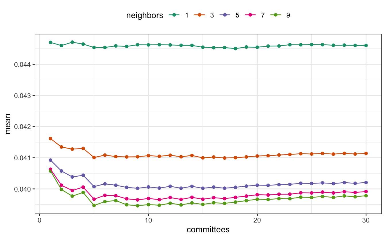
The functions also work with the tune package. To optimize our model, the number of committees (similar to boosting iterations) and the number of nearest-neighbors are the primary parameters for tuning.
cb_grid <- expand.grid(committees = 1:30, neighbors = c(1, 3, 5, 7, 9))

set.seed(8226)
car_folds <- vfold_cv(car_tr)

cubist_mod <-
  cubist_rules(neighbors = tune(), committees = tune()) %>%
  set_engine("Cubist")

car_tune_res <-
  cubist_mod %>%
  tune_grid(log10(Price) ~ ., resamples = car_folds, grid = cb_grid)

car_tune_res %>%
  collect_metrics() %>%
  filter(.metric == "rmse") %>%
  mutate(neighbors = factor(neighbors)) %>%
  ggplot(aes(x = committees, y = mean, col = neighbors)) +
  geom_point() +
  geom_line() +
  scale_color_brewer(palette = "Dark2") +
  theme(legend.position = "top")
show_best(car_tune_res, metric = "rmse")
#> # A tibble: 5 x 7
#>   committees neighbors .metric .estimator   mean     n std_err
#>        <int>     <dbl> <chr>   <chr>       <dbl> <int>   <dbl>
#> 1          9         9 rmse    standard   0.0395    10 0.00133
#> 2          5         9 rmse    standard   0.0395    10 0.00132
#> 3         11         9 rmse    standard   0.0395    10 0.00133
#> 4         13         9 rmse    standard   0.0395    10 0.00132
#> 5          8         9 rmse    standard   0.0395    10 0.00131

smallest_rmse <- select_best(car_tune_res, metric = "rmse")
smallest_rmse
#> # A tibble: 1 x 2
#>   committees neighbors
#>        <int>     <dbl>
#> 1          9         9

final_cb_mod <-
  cubist_mod %>%
  finalize_model(smallest_rmse) %>%
  fit(log10(Price) ~ ., data = car_tr)
It appears that the benefit of using committees occurs in the first 10 iterations. The nearest-neighbor adjustment was important to obtaining good performance.
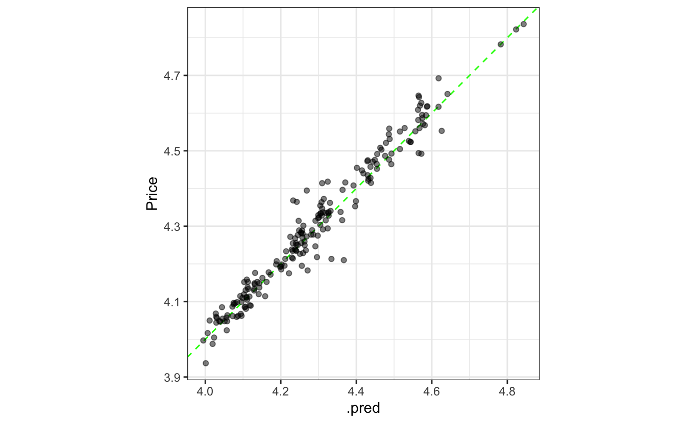
The test set results look good and are consistent with the resampling estimate of RMSE:
test_pred <-
  predict(final_cb_mod, car_te) %>%
  bind_cols(car_te %>% select(Price)) %>%
  mutate(Price = log10(Price))

test_pred %>% rmse(Price, .pred)
#> # A tibble: 1 x 3
#>   .metric .estimator .estimate
#>   <chr>   <chr>          <dbl>
#> 1 rmse    standard      0.0382

ggplot(test_pred, aes(x = .pred, y = Price)) +
  geom_abline(col = "green", lty = 2) +
  geom_point(alpha = 0.5) +
  coord_fixed(ratio = 1)
I’d like to thank Karl Holub for making the xrf package and accepting my PRs and changes.